Visualizers, Displays, and Little Instruments
Field has many ways to show a value, and the quickest takes two keystrokes: put .h on the end of an expression and run the line.
The result might appear inline in the editor, beside the line you ran, or in an output area
under the box. An output area can also become an inspector or a little control panel, with sliders
you can move while the surrounding code keeps running. Let's look at the ways to show and work
with values, starting with .h and .h2.
The value visualizer: what .h draws
Ask Field to show a value and the value visualizer makes a compact HTML view of it. An object becomes a tree you can open; a vector, path or function can also get a small drawing. These three calls reach the same visualizer:
:::static
value.h // the .h extension: value -> pretty HTML
display("inspect", value.h) // drop that HTML into a named output channel
box.viz(value = value) // convenience: visualize into the box's "viz" channel
.h is the lightweight view used throughout Field; its heavier sibling .h2
opens a paged browser for large structures. The built-in and reflective paths are
forgiving: they track recursion by reference, cap depth and preview sizes, catch
reflective getter failures, and guard optional plots and thumbnails (including a
throwing Fn.evalFn). Objects implementing ToHTML and callbacks registered with
registerValuePrinter are extension points whose returned HTML is trusted.
registerValuePrinter is how a third-party type joins in without knowing Field
exists, and the worked example is a Kotlin DataFrame: a frame, a column, a row and a
GroupBy all render as ordinary Field tables, and .h2 pages a million-row frame
through the same offset machinery this page's .h2 uses everywhere else. See
DataFrames in a Box.
The reflective tree
Give the visualizer an ordinary object — a data class, a map, anything with readable properties — and it walks the members into an indented tree. Numbers, booleans, strings, and nested values are each rendered by the same rules, recursively.
:::static
data class Camera(
    val position: Vector3f,
    val fieldOfView: Double,
    val active: Boolean,
    val layers: List<String>,
)

val cam = Camera(Vector3f(0f, 1.5f, -4f), 55.0, true, ["dots", "lines", "labels"])
display("cam", cam.h)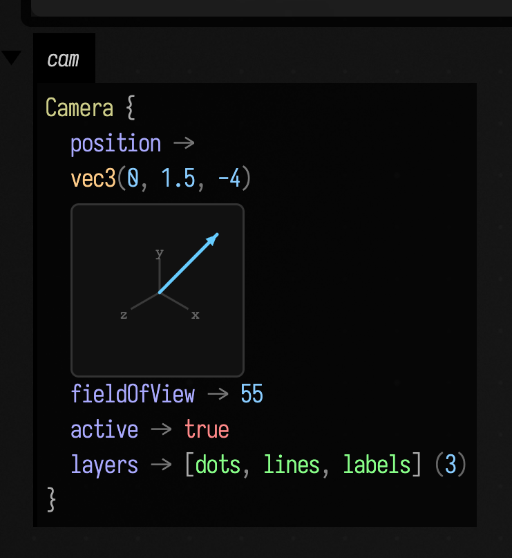
The nested position is drawn as a vec3, and layers collapses to a list with a size count.
For a larger object, open the "… +N more fields" expander to see the rest.
Numeric collections, with stats
Arrays and lists of numbers get a preview plus a one-line statistical summary — mean, standard deviation, and range — so you can judge a buffer without scrolling through it. Long collections elide the middle:
:::static
val samples = DoubleArray(48) { i -> sin(i / 48.0 * 2.0 * Math.PI) }
display("samples", samples.h)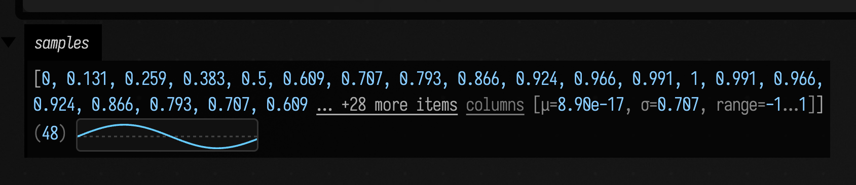
The tail reads … +28 more items [μ=8.90e-17, σ=0.707, range=−1…1] (48): the
sampled sine averages to ~0, has the expected 0.707 RMS spread, and spans −1…1 —
visible immediately, without a plot. The same treatment applies to IntArray,
FloatArray, and numeric Lists.
Vectors, matrices, and quaternions
Vectors render as compact, colour-coded tokens, making their components easy to pick out:
:::static
display("vectors", [vec(0.5, 1.5), vec(1.0, 2.0, 3.0), vec(0.25, 0.5, 1.0, 2.0)].h)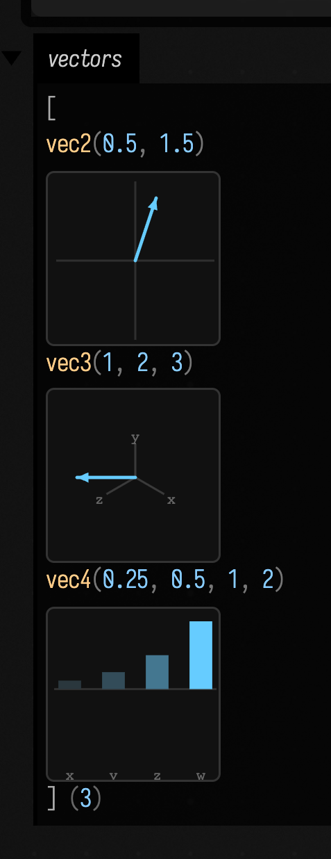
Matrices summarise rather than dump every cell: a mat3 shows its determinant, a
mat4 shows determinant plus extracted translation, and a quaternion shows its
four components. Here they are keyed by a map, which the visualizer renders as a
tree — a good way to label several related values at once:
:::static
display(
    "transforms",
    linkedMapOf(
            "scale (mat3)" to Matrix3f().set(2f, 0f, 0f, 0f, 3f, 0f, 0f, 0f, 1f),
            "translate (mat4)" to
                Matrix4f().identity().apply {
                    set(3, 0, 5f)
                    set(3, 1, -2f)
                    set(3, 2, 1f)
                },
            "spin (quat)" to Quaternionf().rotateY(0.6f),
        )
        .h,
)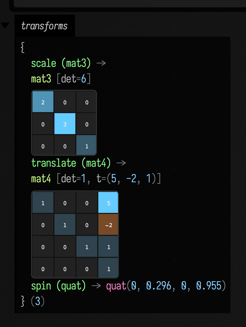
The mat3 reports det=6 (2 × 3 × 1), the mat4 reports det=1, t=(5, -2, 1),
and the quaternion shows its normalized components. For the algebra behind these
types, see Linear Algebra.
An FLine, drawn
For an FLine, Field shows the node counts, bounding box, length and a
compressed path signature, followed by a small SVG drawing of the path:
:::static
val spiral = FLine()
val steps = 140
spiral.breakNext()
for (i in 0..steps) {
    val t = i.toDouble() / steps
    val a = t * 5.0 * 2.0 * Math.PI
    val r = 8.0 + t * 60.0
    val x = 80.0 + Math.cos(a) * r
    val y = 80.0 + Math.sin(a) * r
    spiral.lineTo(x, y)
}
display("spiral", spiral.h)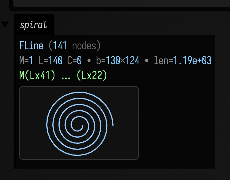
The header reads FLine (141 nodes), then M=1 L=140 C=0 · b=130×124 ·
len=1.19e+03, then the run-compressed signature M(Lx41) … (Lx22), and finally
the thumbnail. The thumbnail is normalised into its box and only rendered for
paths under a complexity budget, so pasting a huge path into a value view never
becomes a rendering hazard.
An Fn, plotted
The richest case is a Functions.Fn. Field keeps the
full reflective tree — its domain, evalFn, graph, and name — because that
graph is the function's rebuildable structure. Then, below it, it appends a safe
SVG line plot of the function sampled over a finite window of its domain:
:::static
with(Functions) {
    val fn = sin(10) over (0.0..3.0)
    display("fn", fn.h)
}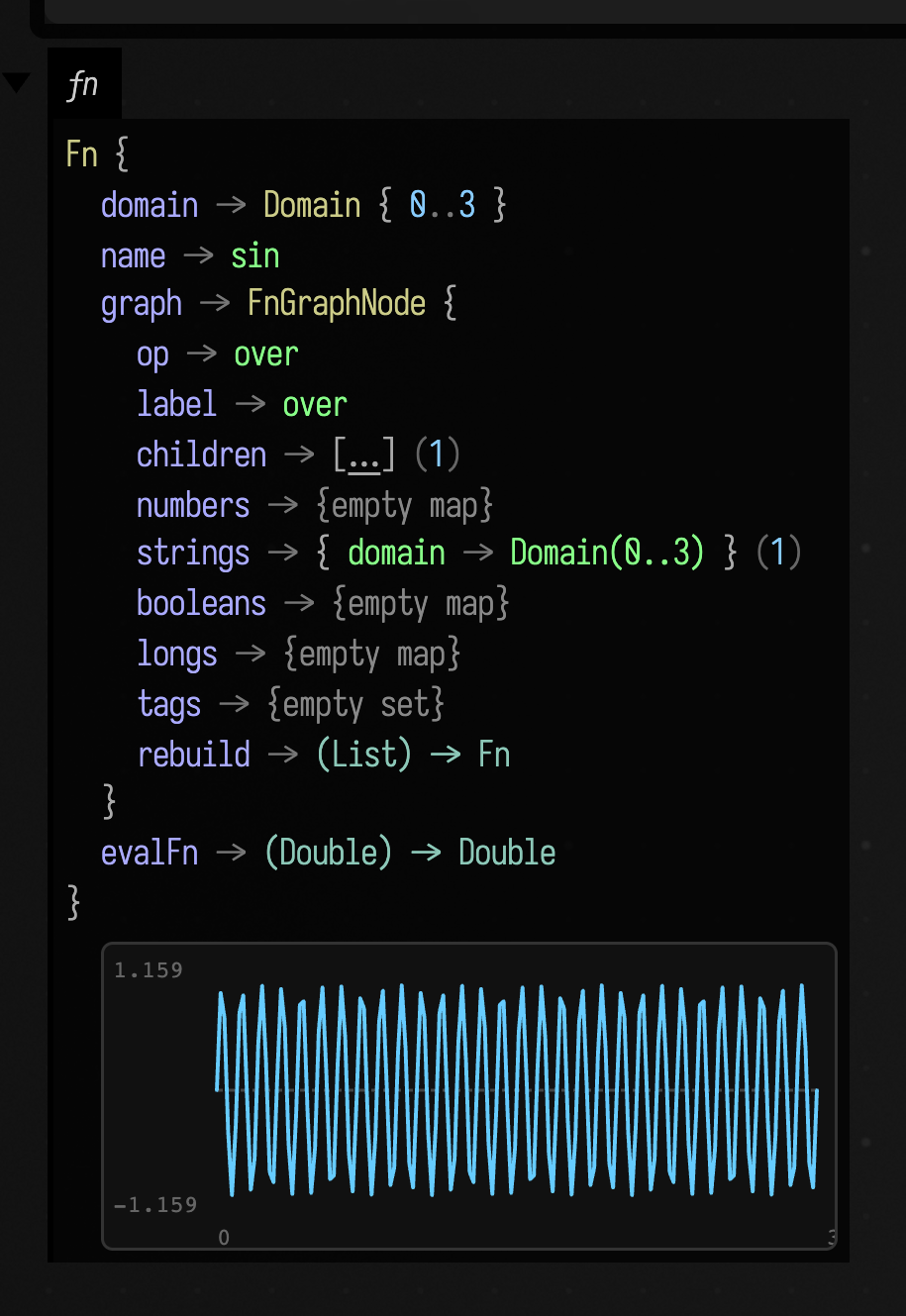
The plot mirrors Fn's own sampling rules: an unbounded domain falls back to a
preview window, non-finite samples become gaps in the curve rather than spikes, a
zero-straddling range draws a dashed baseline, and faint labels mark the value and
domain extents (here 1.159 / −1.159 over 0 … 3). If a function is non-finite
everywhere, or its evalFn throws, the plot is simply omitted and the tree stands
on its own — the value display is never allowed to fail.
Images, edges, corners and flow
The same .h also helps you look at images and computer-vision results.
Instead of reading a long array or a list of coordinates, you can see the pixels, detected corners,
gradients or motion directly.
Evaluate an Img and you get the actual pixels, aspect-correct, plus a <details>
disclosure holding the per-channel strip, a per-channel histogram computed over the
full-resolution samples, and the numbers:
:::static
:::fold the scene: a gradient, a bright rectangle, a disc, two rulings and a checker patch
val scene =
    Img.generateRGB(240, 180) { x, y ->
        var r = 0.10f + 0.30f * (x / 239f)
        var g = 0.12f + 0.22f * (y / 179f)
        var b = 0.34f - 0.20f * (x / 239f)
        if (x in 30..90 && y in 26..76) {
            r = 0.94f
            g = 0.86f
            b = 0.42f
        }
        if (hypot(x - 172.0, y - 62.0) <= 30.0) {
            r = 0.30f
            g = 0.80f
            b = 0.92f
        }
        if (x in 150..152 || y in 140..142) {
            r = 0.98f
            g = 0.98f
            b = 0.98f
        }
        if (x in 24..104 && y in 104..164 && (x / 8 + y / 8) % 2 == 0) {
            r = 0.88f
            g = 0.30f
            b = 0.55f
        }
        Triple(r, g, b)
    }
:::endfold
display("scene", scene.h)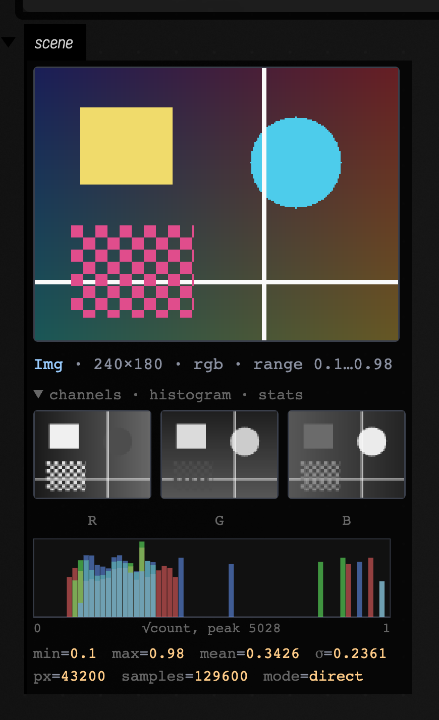
The range policy
Image channels can contain values outside 0…1: a Sobel dx has negative values, for example,
and an unnormalised response can exceed 1. The visualizer chooses a display range for the data
and names the mode it used:
direct — every finite sample is already in 0…1. Nothing is rescaled, and the
caption says direct. That is the picture above.
signed ±m — some sample is negative. The range is made symmetric about zero, so
that zero is a fixed, recognisable colour rather than wherever min…max happened
to put it, and a 1-channel image is run through the coolwarm diverging ramp from
Colormaps — blue negative, pale zero, red positive.
Grey simply cannot carry a sign:
:::static
:::fold the scene: a gradient, a bright rectangle, a disc, two rulings and a checker patch
val scene =
    Img.generateRGB(240, 180) { x, y ->
        var r = 0.10f + 0.30f * (x / 239f)
        var g = 0.12f + 0.22f * (y / 179f)
        var b = 0.34f - 0.20f * (x / 239f)
        if (x in 30..90 && y in 26..76) {
            r = 0.94f
            g = 0.86f
            b = 0.42f
        }
        if (hypot(x - 172.0, y - 62.0) <= 30.0) {
            r = 0.30f
            g = 0.80f
            b = 0.92f
        }
        if (x in 150..152 || y in 140..142) {
            r = 0.98f
            g = 0.98f
            b = 0.98f
        }
        if (x in 24..104 && y in 104..164 && (x / 8 + y / 8) % 2 == 0) {
            r = 0.88f
            g = 0.30f
            b = 0.55f
        }
        Triple(r, g, b)
    }
:::endfold
display("dx", scene.luma().sobel().dx.h)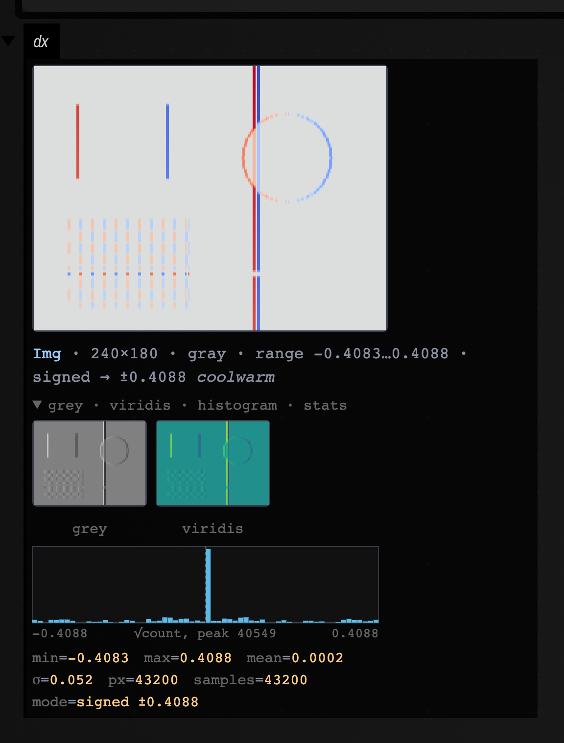
Read it: the rectangle's left edge is red (dark→bright going right, so dx > 0)
and its right edge is blue; the disc is warm on its left limb and cool on its
right. mean = 0.0002 and σ = 0.052, with the histogram spiking at zero, is what
a gradient of a mostly-flat image should look like. The disclosure offers the same
data read two more ways — plain grey and viridis — so you get three readings of
one response image.
auto-ranged — non-negative, but the maximum is above 1. Rescaled for display
with the true range printed, so a bright pixel is never mistaken for 1.0:
:::static
:::fold the scene: a gradient, a bright rectangle, a disc, two rulings and a checker patch
val scene =
    Img.generateRGB(240, 180) { x, y ->
        var r = 0.10f + 0.30f * (x / 239f)
        var g = 0.12f + 0.22f * (y / 179f)
        var b = 0.34f - 0.20f * (x / 239f)
        if (x in 30..90 && y in 26..76) {
            r = 0.94f
            g = 0.86f
            b = 0.42f
        }
        if (hypot(x - 172.0, y - 62.0) <= 30.0) {
            r = 0.30f
            g = 0.80f
            b = 0.92f
        }
        if (x in 150..152 || y in 140..142) {
            r = 0.98f
            g = 0.98f
            b = 0.98f
        }
        if (x in 24..104 && y in 104..164 && (x / 8 + y / 8) % 2 == 0) {
            r = 0.88f
            g = 0.30f
            b = 0.55f
        }
        Triple(r, g, b)
    }
:::endfold
display("edges", (scene.luma().sobelMagnitude() * 25f).h)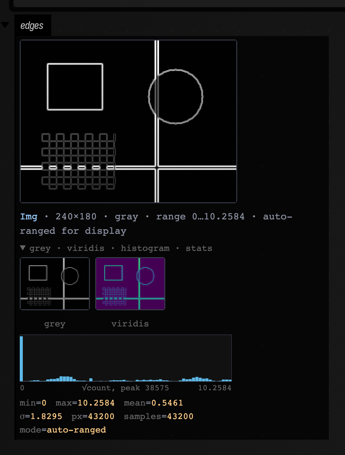
And non-finite samples — NaN, ±∞ — are counted, excluded from every statistic, and painted magenta:
:::static
val ramp =
    Img.generate(96, 72) { x, y ->
        when {
            x in 40..47 && y in 30..37 -> Float.NaN
            x == 70 && y == 20 -> Float.POSITIVE_INFINITY
            else -> (x + y) / 166f
        }
    }
display("ramp", ramp.h)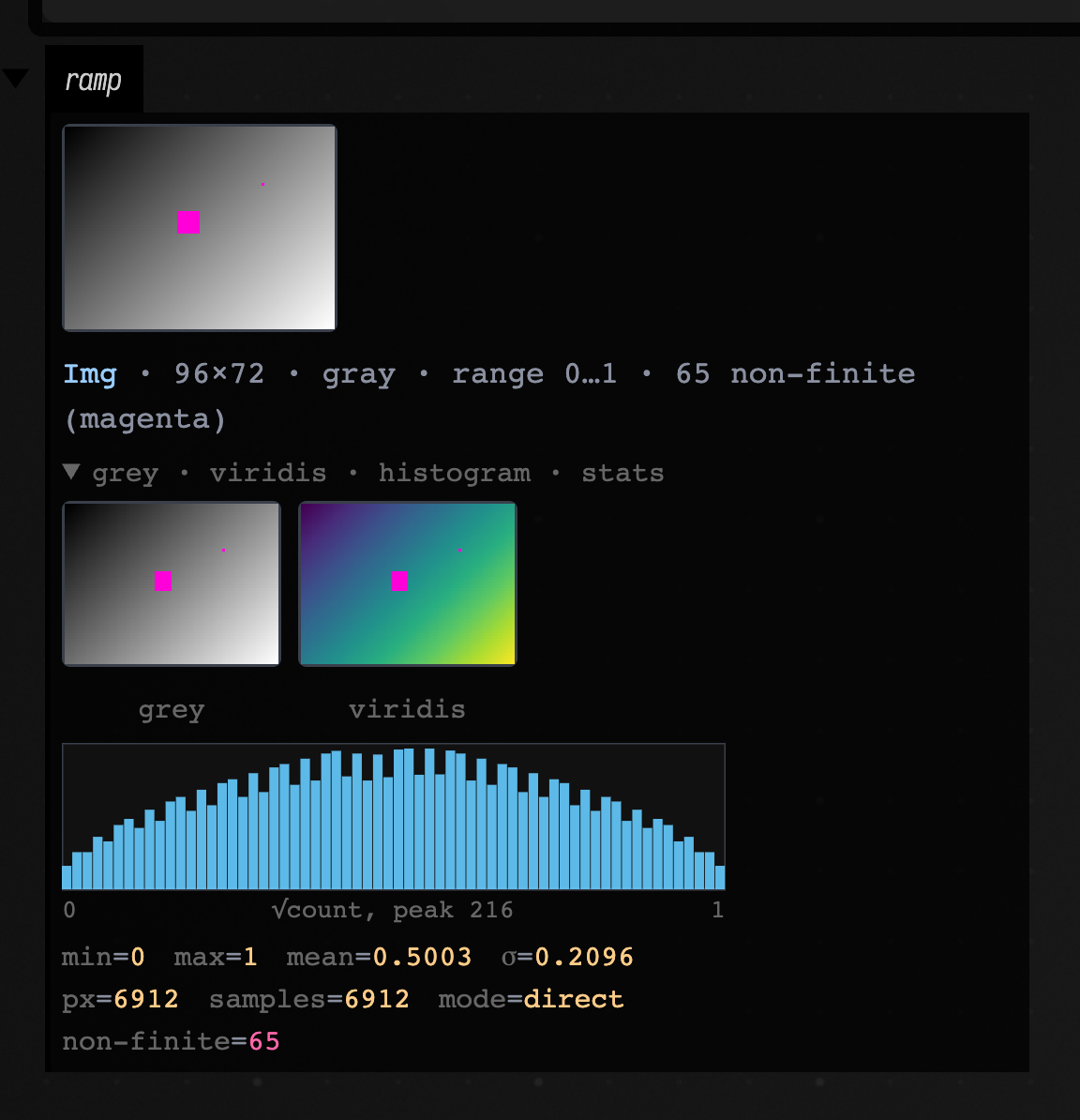
The magenta pixels make missing or invalid values visible, and the count tells you how many samples need attention.
Four-channel images sit on a checkerboard, so transparent black and opaque black are different pictures:
:::static
val w = 140
val h = 140
val data = FloatArray(w * h * 4)
for (y in 0 until h) for (x in 0 until w) {
    val i = (y * w + x) * 4
    data[i] = 0.95f
    data[i + 1] = 0.55f
    data[i + 2] = 0.20f
    data[i + 3] = (1.0 - hypot(x - 70.0, y - 70.0) / 66.0).coerceIn(0.0, 1.0).toFloat()
}
display("glow", Img(w, h, 4, data).h)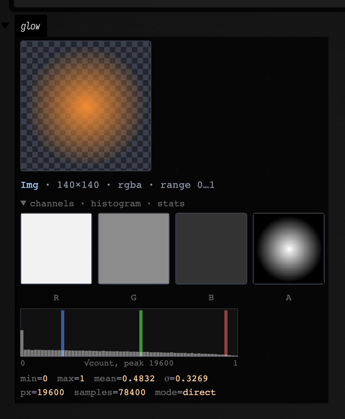
Gradients and pyramids
A Gradient is two signed images and a direction, so it shows all of it — dx,
dy, the magnitude, and the hue-by-direction image the type already knows how to
build:
:::static
:::fold the scene: a gradient, a bright rectangle, a disc, two rulings and a checker patch
val scene =
    Img.generateRGB(240, 180) { x, y ->
        var r = 0.10f + 0.30f * (x / 239f)
        var g = 0.12f + 0.22f * (y / 179f)
        var b = 0.34f - 0.20f * (x / 239f)
        if (x in 30..90 && y in 26..76) {
            r = 0.94f
            g = 0.86f
            b = 0.42f
        }
        if (hypot(x - 172.0, y - 62.0) <= 30.0) {
            r = 0.30f
            g = 0.80f
            b = 0.92f
        }
        if (x in 150..152 || y in 140..142) {
            r = 0.98f
            g = 0.98f
            b = 0.98f
        }
        if (x in 24..104 && y in 104..164 && (x / 8 + y / 8) % 2 == 0) {
            r = 0.88f
            g = 0.30f
            b = 0.55f
        }
        Triple(r, g, b)
    }
:::endfold
display("gradient", scene.luma().sobel().h)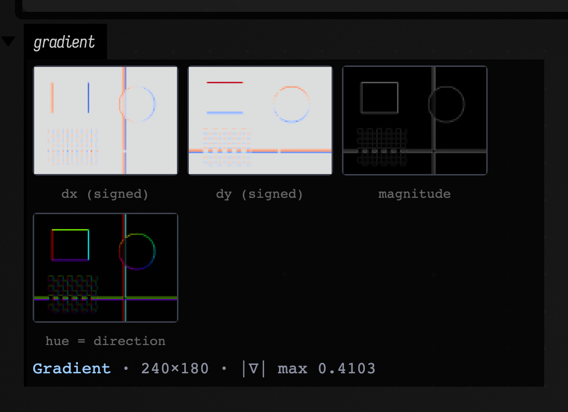
A pyramid is drawn as a ladder of rungs at true relative scale, bottom-aligned, so you can see each level halve in size:
:::static
:::fold the scene: a gradient, a bright rectangle, a disc, two rulings and a checker patch
val scene =
    Img.generateRGB(240, 180) { x, y ->
        var r = 0.10f + 0.30f * (x / 239f)
        var g = 0.12f + 0.22f * (y / 179f)
        var b = 0.34f - 0.20f * (x / 239f)
        if (x in 30..90 && y in 26..76) {
            r = 0.94f
            g = 0.86f
            b = 0.42f
        }
        if (hypot(x - 172.0, y - 62.0) <= 30.0) {
            r = 0.30f
            g = 0.80f
            b = 0.92f
        }
        if (x in 150..152 || y in 140..142) {
            r = 0.98f
            g = 0.98f
            b = 0.98f
        }
        if (x in 24..104 && y in 104..164 && (x / 8 + y / 8) % 2 == 0) {
            r = 0.88f
            g = 0.30f
            b = 0.55f
        }
        Triple(r, g, b)
    }
:::endfold
display("pyramid", scene.gaussianPyramid(5).h)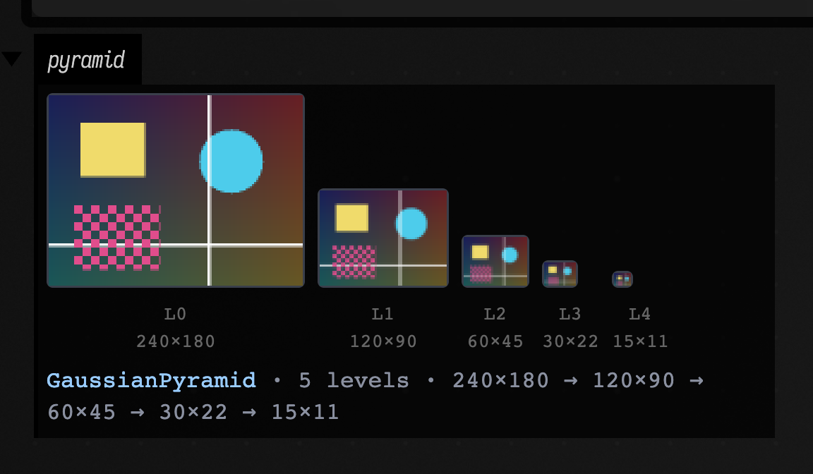
:::static
:::fold the scene: a gradient, a bright rectangle, a disc, two rulings and a checker patch
val scene =
    Img.generateRGB(240, 180) { x, y ->
        var r = 0.10f + 0.30f * (x / 239f)
        var g = 0.12f + 0.22f * (y / 179f)
        var b = 0.34f - 0.20f * (x / 239f)
        if (x in 30..90 && y in 26..76) {
            r = 0.94f
            g = 0.86f
            b = 0.42f
        }
        if (hypot(x - 172.0, y - 62.0) <= 30.0) {
            r = 0.30f
            g = 0.80f
            b = 0.92f
        }
        if (x in 150..152 || y in 140..142) {
            r = 0.98f
            g = 0.98f
            b = 0.98f
        }
        if (x in 24..104 && y in 104..164 && (x / 8 + y / 8) % 2 == 0) {
            r = 0.88f
            g = 0.30f
            b = 0.55f
        }
        Triple(r, g, b)
    }
:::endfold
display("bands", scene.luma().laplacianPyramid(4).h)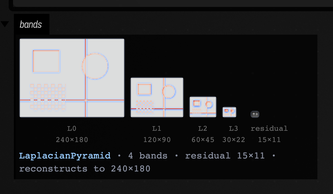
The Laplacian bands are signed, so they get the diverging treatment, and the one
rung that is not a band is labelled residual.
Detector output
A List<Corner> becomes a scatter with detector strength as both radius and
viridis colour. A corner list carries no image extent, so the canvas is the
points' own bounding box unioned with the origin — image coordinates start at
(0, 0), and including it keeps the points where they actually sit in the frame.
The caption states the inferred extent:
:::static
:::fold the scene: a gradient, a bright rectangle, a disc, two rulings and a checker patch
val scene =
    Img.generateRGB(240, 180) { x, y ->
        var r = 0.10f + 0.30f * (x / 239f)
        var g = 0.12f + 0.22f * (y / 179f)
        var b = 0.34f - 0.20f * (x / 239f)
        if (x in 30..90 && y in 26..76) {
            r = 0.94f
            g = 0.86f
            b = 0.42f
        }
        if (hypot(x - 172.0, y - 62.0) <= 30.0) {
            r = 0.30f
            g = 0.80f
            b = 0.92f
        }
        if (x in 150..152 || y in 140..142) {
            r = 0.98f
            g = 0.98f
            b = 0.98f
        }
        if (x in 24..104 && y in 104..164 && (x / 8 + y / 8) % 2 == 0) {
            r = 0.88f
            g = 0.30f
            b = 0.55f
        }
        Triple(r, g, b)
    }
:::endfold
display("corners", scene.luma().harrisCorners(minDistance = 8, maxCount = 40).h)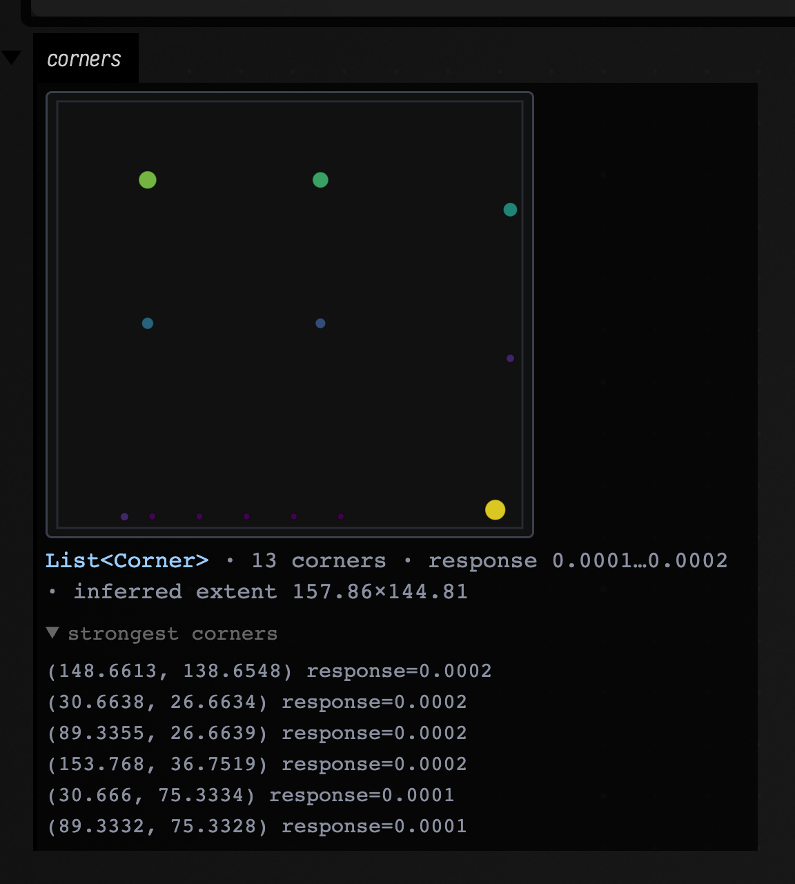
The strongest corner, (148.7, 138.7), is where the two rulings cross. Next come
(30.7, 26.7) and (89.3, 26.7), and further down the list (30.7, 75.3) and
(89.3, 75.3): the four corners of the rectangle planted at x 30…90, y 26…76.
A HoughLine is (rho, theta): an infinite line with no extent of its own,
which is why toFLine insists on being handed the image dimensions. With no image
in reach the left panel clips each line into the smallest square every peak can
still cross, says which square that was, and points at linesToFLines for the
in-place version. The right panel needs no extent at all and is therefore exact:
ρ against θ, sized by votes.
:::static
:::fold the scene: a gradient, a bright rectangle, a disc, two rulings and a checker patch
val scene =
    Img.generateRGB(240, 180) { x, y ->
        var r = 0.10f + 0.30f * (x / 239f)
        var g = 0.12f + 0.22f * (y / 179f)
        var b = 0.34f - 0.20f * (x / 239f)
        if (x in 30..90 && y in 26..76) {
            r = 0.94f
            g = 0.86f
            b = 0.42f
        }
        if (hypot(x - 172.0, y - 62.0) <= 30.0) {
            r = 0.30f
            g = 0.80f
            b = 0.92f
        }
        if (x in 150..152 || y in 140..142) {
            r = 0.98f
            g = 0.98f
            b = 0.98f
        }
        if (x in 24..104 && y in 104..164 && (x / 8 + y / 8) % 2 == 0) {
            r = 0.88f
            g = 0.30f
            b = 0.55f
        }
        Triple(r, g, b)
    }
:::endfold
val edges = scene.luma().canny(0.10, 0.25)
display("lines", houghLines(edges, maxLines = 8, threshold = 40).h)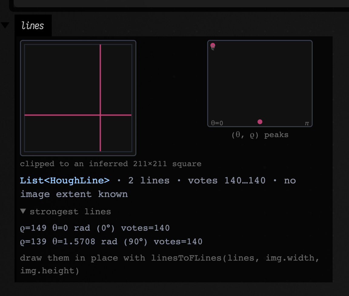
A circle does have an extent, so no assumption is needed:
:::static
:::fold the scene: a gradient, a bright rectangle, a disc, two rulings and a checker patch
val scene =
    Img.generateRGB(240, 180) { x, y ->
        var r = 0.10f + 0.30f * (x / 239f)
        var g = 0.12f + 0.22f * (y / 179f)
        var b = 0.34f - 0.20f * (x / 239f)
        if (x in 30..90 && y in 26..76) {
            r = 0.94f
            g = 0.86f
            b = 0.42f
        }
        if (hypot(x - 172.0, y - 62.0) <= 30.0) {
            r = 0.30f
            g = 0.80f
            b = 0.92f
        }
        if (x in 150..152 || y in 140..142) {
            r = 0.98f
            g = 0.98f
            b = 0.98f
        }
        if (x in 24..104 && y in 104..164 && (x / 8 + y / 8) % 2 == 0) {
            r = 0.88f
            g = 0.30f
            b = 0.55f
        }
        Triple(r, g, b)
    }
:::endfold
val edges = scene.luma().canny(0.10, 0.25)
display("circles", houghCircles(edges, minRadius = 20, maxRadius = 40, maxCircles = 4).h)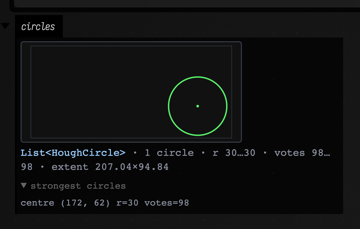
A FlowField shows one arrow per converged track, coloured by direction; grey crosses mark tracks
that failed. Displacements are drawn at their pixel scale unless the median motion is too small to
see. In that case the view enlarges them and reports the factor:
:::static
:::fold the scene: a gradient, a bright rectangle, a disc, two rulings and a checker patch
val scene =
    Img.generateRGB(240, 180) { x, y ->
        var r = 0.10f + 0.30f * (x / 239f)
        var g = 0.12f + 0.22f * (y / 179f)
        var b = 0.34f - 0.20f * (x / 239f)
        if (x in 30..90 && y in 26..76) {
            r = 0.94f
            g = 0.86f
            b = 0.42f
        }
        if (hypot(x - 172.0, y - 62.0) <= 30.0) {
            r = 0.30f
            g = 0.80f
            b = 0.92f
        }
        if (x in 150..152 || y in 140..142) {
            r = 0.98f
            g = 0.98f
            b = 0.98f
        }
        if (x in 24..104 && y in 104..164 && (x / 8 + y / 8) % 2 == 0) {
            r = 0.88f
            g = 0.30f
            b = 0.55f
        }
        Triple(r, g, b)
    }
:::endfold
val before = scene.luma()
val after = scene.rotate(0.06).luma()
val seeds = before.goodFeaturesToTrack(maxCount = 90, minDistance = 9)
display("flow", opticalFlowLK(before, after, seeds.map { it.toVec2() }, levels = 3).h)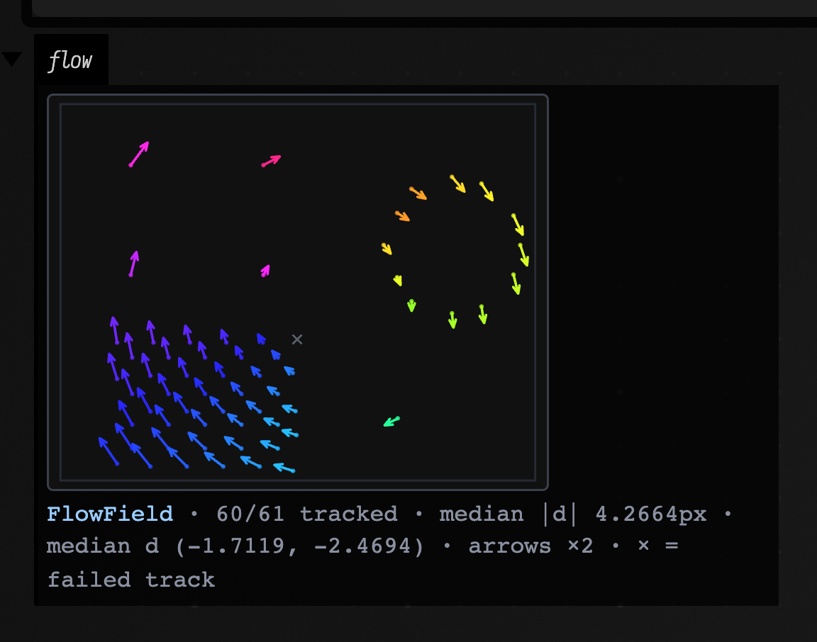
The frames here differ by a 0.06 rad rotation about the centre, and that is exactly what the arrows trace: little motion near the middle, tangential motion at the edges, the hue rotating smoothly with the direction.
Finally, a ComponentLabelling shows the label map under a golden-ratio hue
rotation — adjacent label ids get unrelated colours, which is what makes two
touching blobs distinguishable at thumbnail size — with the per-blob areas and
centroids behind the disclosure:
:::static
:::fold the scene: a gradient, a bright rectangle, a disc, two rulings and a checker patch
val scene =
    Img.generateRGB(240, 180) { x, y ->
        var r = 0.10f + 0.30f * (x / 239f)
        var g = 0.12f + 0.22f * (y / 179f)
        var b = 0.34f - 0.20f * (x / 239f)
        if (x in 30..90 && y in 26..76) {
            r = 0.94f
            g = 0.86f
            b = 0.42f
        }
        if (hypot(x - 172.0, y - 62.0) <= 30.0) {
            r = 0.30f
            g = 0.80f
            b = 0.92f
        }
        if (x in 150..152 || y in 140..142) {
            r = 0.98f
            g = 0.98f
            b = 0.98f
        }
        if (x in 24..104 && y in 104..164 && (x / 8 + y / 8) % 2 == 0) {
            r = 0.88f
            g = 0.30f
            b = 0.55f
        }
        Triple(r, g, b)
    }
:::endfold
display("blobs", scene.luma().gaussianBlur(1.2).thresholdOtsu().connectedComponents().h)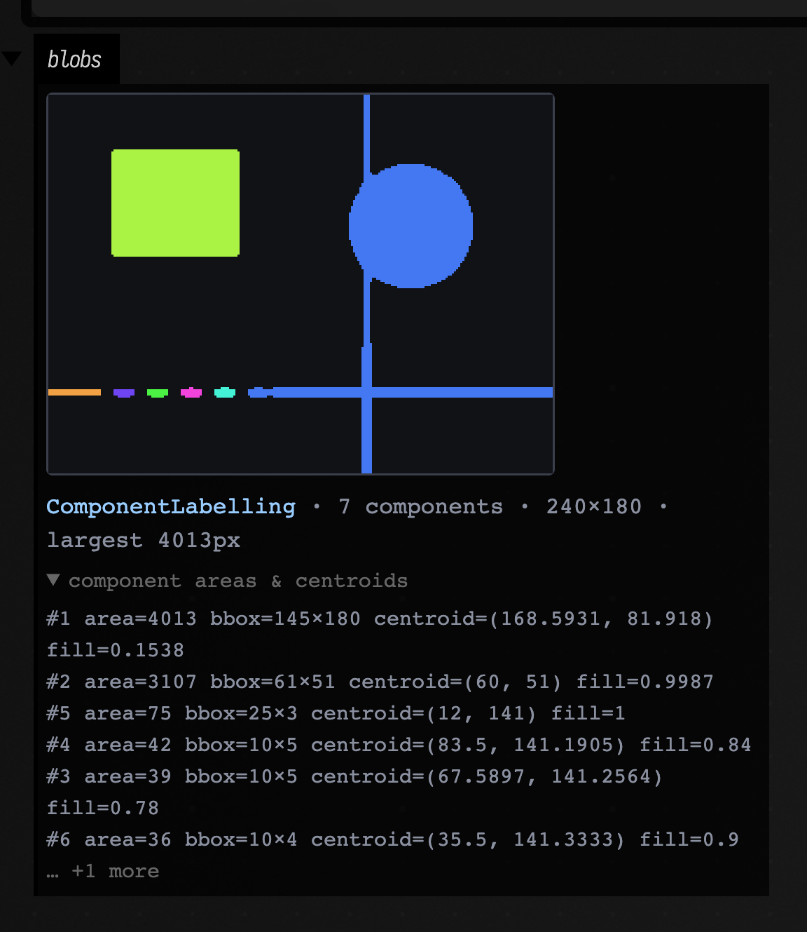
A plain List<Img> becomes a filmstrip, which is the shape a frame sequence or a
parameter sweep already has:
:::static
:::fold the scene: a gradient, a bright rectangle, a disc, two rulings and a checker patch
val scene =
    Img.generateRGB(240, 180) { x, y ->
        var r = 0.10f + 0.30f * (x / 239f)
        var g = 0.12f + 0.22f * (y / 179f)
        var b = 0.34f - 0.20f * (x / 239f)
        if (x in 30..90 && y in 26..76) {
            r = 0.94f
            g = 0.86f
            b = 0.42f
        }
        if (hypot(x - 172.0, y - 62.0) <= 30.0) {
            r = 0.30f
            g = 0.80f
            b = 0.92f
        }
        if (x in 150..152 || y in 140..142) {
            r = 0.98f
            g = 0.98f
            b = 0.98f
        }
        if (x in 24..104 && y in 104..164 && (x / 8 + y / 8) % 2 == 0) {
            r = 0.88f
            g = 0.30f
            b = 0.55f
        }
        Triple(r, g, b)
    }
:::endfold
display("sweep", (0 until 5).map { i -> scene.gaussianBlur(0.001 + i * 1.6) }.h)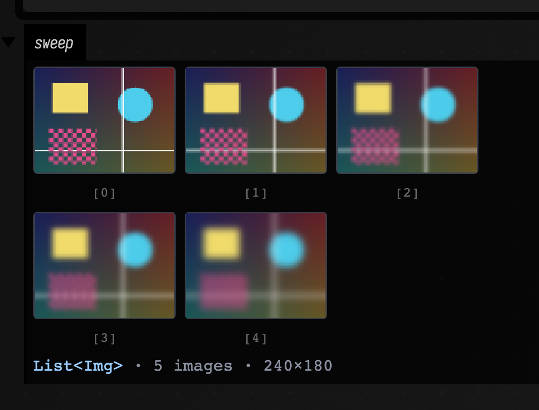
A whole pipeline in one box
Each figure above is one value in its own box. Several values can share one output channel: here
four stages of a pipeline sit in two rows of two, with .h doing all the work.
:::static
val scene =
    Img.generateRGB(180, 132) { x, y ->
        var r = 0.10f + 0.30f * (x / 179f)
        var g = 0.12f + 0.22f * (y / 131f)
        var b = 0.34f - 0.20f * (x / 179f)
        if (x in 24..68 && y in 20..56) {
            r = 0.94f
            g = 0.86f
            b = 0.42f
        }
        if (hypot(x - 128.0, y - 46.0) <= 22.0) {
            r = 0.30f
            g = 0.80f
            b = 0.92f
        }
        if (x in 112..113 || y in 104..105) {
            r = 0.98f
            g = 0.98f
            b = 0.98f
        }
        Triple(r, g, b)
    }
val gray = scene.luma()

// Four stages of one pipeline, four different value types, one `.h` each, laid out as
// two rows of two in a single output channel.
val panels = [
    scene.h, // direct mode, 3 channels
    gray.sobel().dx.h, // signed -> coolwarm diverging
    gray.gaussianPyramid(4).h, // rungs at true relative scale
    gray.harrisCorners(minDistance = 6, maxCount = 20).h, // scatter, strength-coded
]
markdown("panels", FieldMarkdown.row(panels.take(2)) + "\n\n" + FieldMarkdown.row(panels.drop(2)))

println("imaging visualizers ready")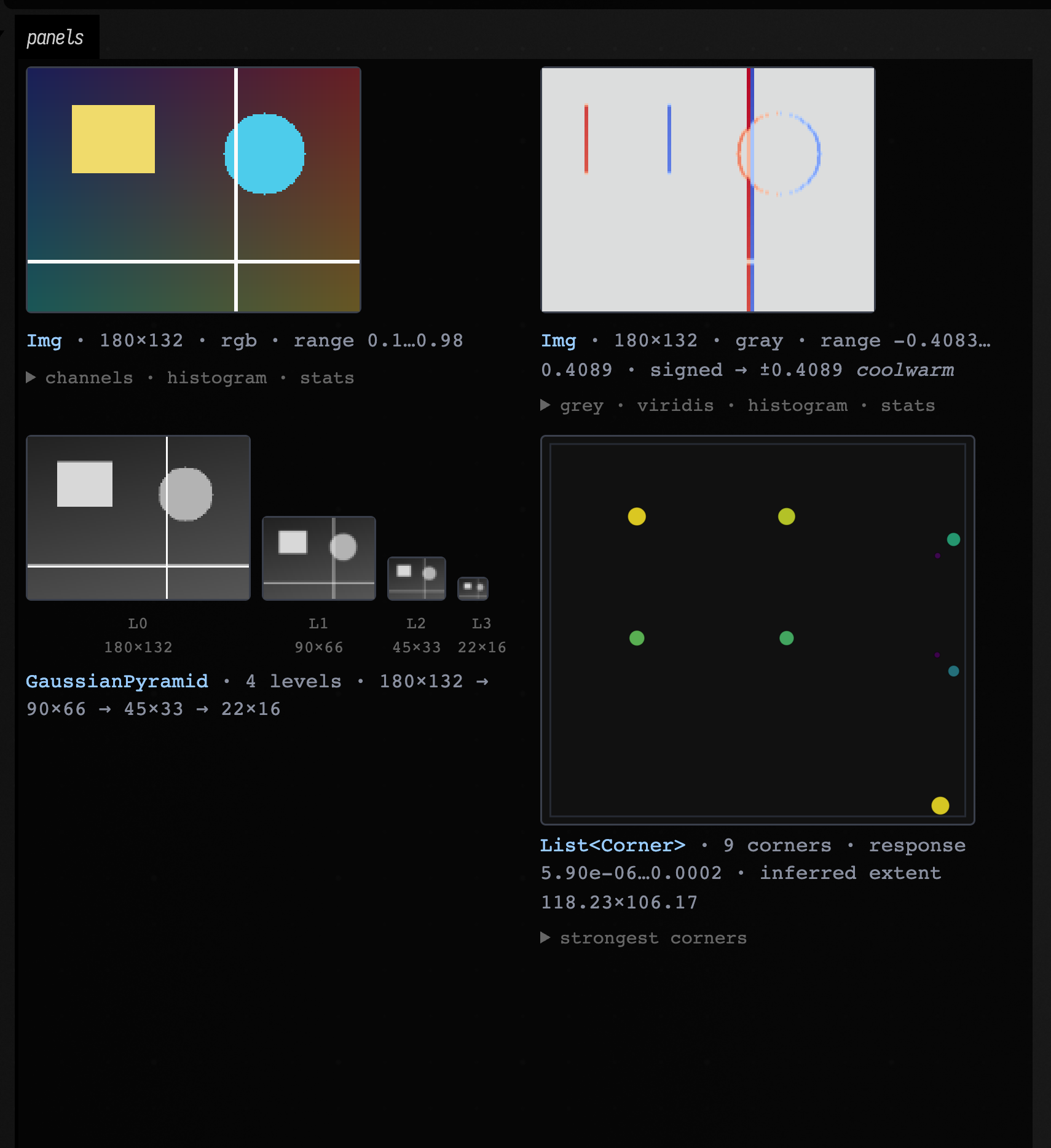
Each value ends in .h. Field chooses a view suited to it, whether it is colour data, a signed
response, a pyramid or a list of detections.
Open the demo document
The imaging_visualizers_demo
starting point has one box per visualizer on this page. Open it from the
welcome screen, run the boxes and look at each one's output area. Each box
ends with one imaging value, and Field draws it; no display(...) call is
needed. Then change a sigma or a threshold and re-run a box.
Next, let's put visualizers beside running code, display larger results under a box, and add controls you can move while the code runs.
Inline editor visualizers
These draw next to the line of code that produced the value. The core pattern is:
:::static
val m = __m("some-marker")
m.histogram(0.42)
The marker keeps the values it needs and draws the result beside that line in the editor.
Histogram, history, and summary stats
Histograms answer “what values have I seen?”, history answers “how did the value move?”, and stats gives you a one-line summary.
The live examples below are all loop { } bodies, which is Field's frame loop: the body runs, then
the frame advances, once per Runloop tick. What that tick is, and what stops one of these, is
Frames and the animation loop.
:::static
var tick = 0.0
var visualizerFrame = 0

println("inline metrics ready")

loop {
    tick += 0.4
    visualizerFrame += 1

    if (visualizerFrame % 2 == 0) {
        val value = sin(tick * 0.22) * 0.7 + cos(tick * 0.11) * 0.2 + tick * 0.01

        __m("histogram").histogram(value, dur = 120)
        __m("trail").history(value, dur = 48)
        __m("summary").stats(value, dur = 48)
    }
    frame()
}
Those three calls all share the same basic idea:
ᛟ.histogram(value)keeps a rolling distribution.ᛟ.history(value)keeps a rolling time series.ᛟ.stats(value)gives a compact summary panel.
In the editor you can add a marker rune (ᛟ), with f1, "Insert Stack Mark", or shift+command period:
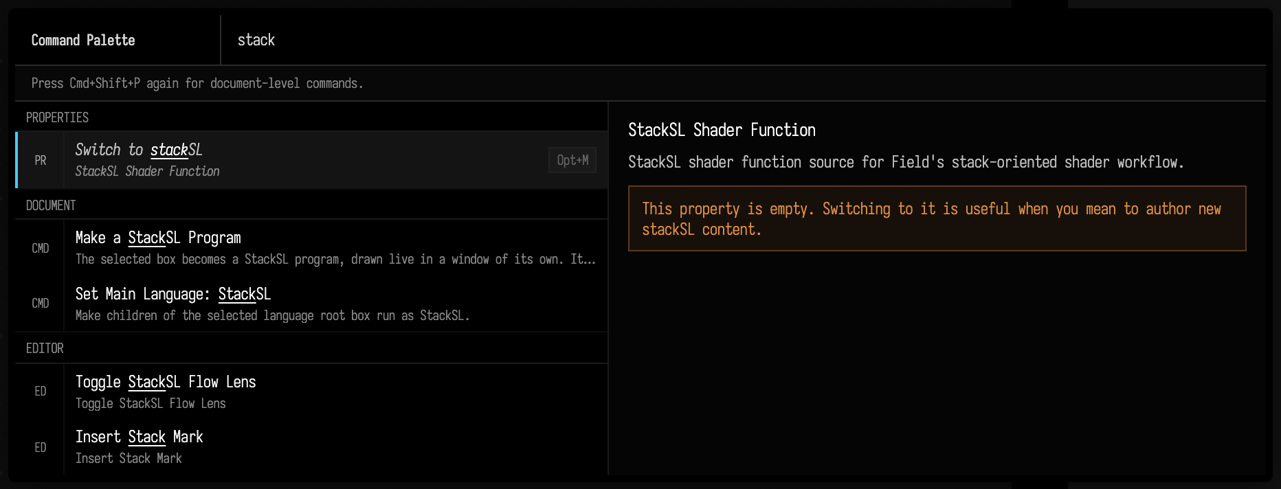
These functions are passthroughs. They return the value they were given, so you can drop them into a chain when you want to inspect the value flowing through a wire without changing the computation:
:::static
val filtered = __m("cutoff").history(rawCutoff)
They make handy little scopes for seeing a value as it passes through your code.
If you want a live feed rather than a one-shot summary, write a loop and launch the box:
:::static
println("live history launched")

var phase = 0.0
var visualizerFrame = 0

loop {
    visualizerFrame += 1
    if (visualizerFrame % 2 == 0) {
        val y = sin(phase * 0.8) + 0.2 * sin(phase * 7.0)
        __m("live").history(y, dur = 120)
    }
    phase += 0.07
    frame()
}
The same loop is shorter written against the box's time instead of a phase it advances itself:
:::static
loop {
    val t = time
    val y = sin(t * 0.8) + 0.2 * sin(t * 7.0)
    __m("live").history(y, dur = 120)
    frame()
}
Run either as a launch, not a plain execute.
Piano rolls in the editor
The piano-roll visualizer is the same idea, but for scheduled notes rather than scalar values.
:::static
val arp = noteProcess {
    val chord = [48, 55, 60, 64]
    var step = 0
    while (true) {
        note(
            pitch = chord[step % chord.size],
            duration = 0.18,
            velocity = 0.85,
            label = "n$step",
        )
        rest(0.25)
        step++
    }
}

println("inline piano roll launched")

var playhead = 0.0
var visualizerFrame = 0

loop {
    visualizerFrame += 1
    if (visualizerFrame % 2 == 0) {
        __m("arp").pianoRoll(arp.at(playhead))
    }
    playhead += 0.35
    frame()
}
Use it for sequencers, generative rhythm systems, or anything where you want to see future note structure without leaving the code.
Display channels: the big canvas under the box
Inline visuals sit beside one line of code. display(...) has the whole area under the box.
Anything you pass to display("channel", thing) becomes HTML in a named output area. That HTML can be handwritten, auto-generated, interactive, or even an embedded browser/inspector.
Raw HTML, pretty HTML, and heavy HTML
display("channel", "<div>...</div>")is the raw escape hatch..hturns a value into a lightweight pretty HTML view..h2turns a heavier structure into a paged browser / explorer.
:::static
val tiny = linkedMapOf(
    "tempo" to 122,
    "mode" to "mixolydian",
    "active" to true,
    "notes" to ["C", "E", "G", "Bb"],
)

val big =
    (0 until 18).associate { row ->
        "row-$row" to
            (0 until 10).associate { col ->
                "c$col" to row * col
            }
    }

display(
    "hello",
    "<div style=\"padding:18px;background:#101820;color:#f2aa4c;border:1px solid #2d4a5d\">" +
        "<b>display(...)</b> can show any HTML you like." +
        "</div>",
)
display("pretty", tiny.h)
display("heavy", big.h2)

println("display helpers ready")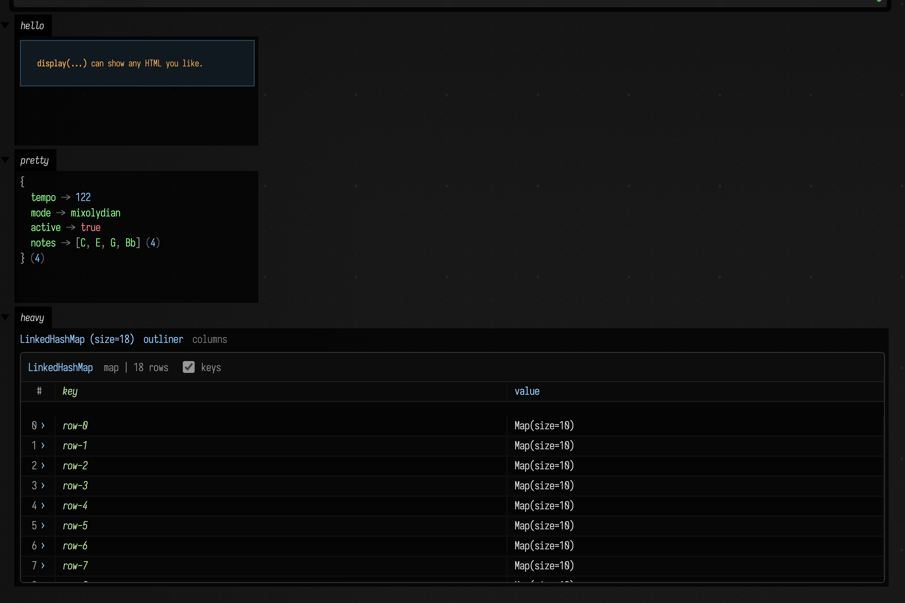
Use .h for a compact view, and .h2 when you want to browse a larger map, list, array or buffer.
Both work with your own data classes as well as Field's types.
.h2 on a plain object gives you its properties as a scrollable table: one row per property, with its declared type and its value. Above the table sit outliner and columns links, which open the same value in the full tree and column browsers. There is nothing to register; it reflects. If a property's getter throws, the row is still there, marked, with the exception text in its value cell.
Four things are special-cased, because their fields are not where the interesting content is. A Box shows its name, frame, code size, run state, its whole property bag, and a table of its parents, children, nested and nestedIn edges. An Fn shows a sampled table of x and f(x) across its domain, because a function is its values and its one substantive field is a private closure. An FLine shows its node table: instruction kind, control-point count and endpoint per row. An exception shows its message, its cause chain and its stack.
Some values .h2 hands straight back to .h, because the compact rendering already is the value: numbers, strings, enums, a Pair, a vector, a matrix (which .h draws as a heatmap), and a Quantity, whose whole point is a number next to a unit.
To see all of it at once, insert the h2 Explorer Examples template and run its boxes top to bottom.
Markdown for captions and tables
For a heading, a table and some text, Markdown is often easier to write than a string of HTML.
markdown("channel", "…") displays it using Field's styles:
:::static
val readings = linkedMapOf("tempo" to 122, "drift" to -0.004, "voice" to "saw 110 *")
val rows = readings.entries.joinToString("\n") { (k, v) -> "| ${k.md} | ${v.md} |" }
val report = "converged in 41 steps\nresidual 3.2e-7"

markdown(
    "figure",
    """
    ### what the run settled on

    | reading | value |
    |---------|-------|
    $rows

    status: {ok:**stable**} · budget: {warn:83% used} · {muted:no retries}

    :::row
    #### before
    ${mapOf("gain" to 0.2).h}
    ---
    #### after
    ${mapOf("gain" to 0.9).h}
    :::end

    #### solver output
    ~~~
$report
    ~~~
""",
    width = 820,
)

println("markdown figure ready")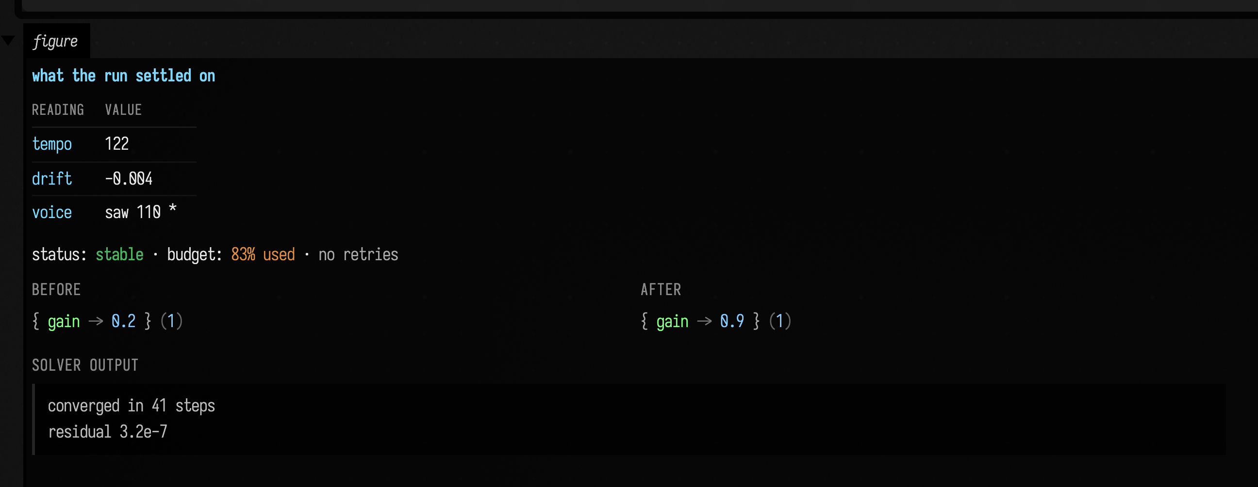
Three rules matter once a figure mixes computed values into the prose:
- HTML passes through, inline and block.
.h,diffHtml(),graphSvg()and friends already return HTML; interpolate them directly and they land verbatim, table cells included. Only text you actually wrote as markdown gets escaped. value.mdfor computed values. Runtime values are not markdown — a|splits the row it lands in, a pair of*becomes emphasis, a<b>is read as a tag and vanishes. Escape anything you did not write yourself.mdEscape(value)is the same function, written as a call.- Fenced bodies are interpolated at column zero, hard left, the way
$reportis above. Inside a fence whitespace is the content, and splicing at the surrounding indentation would indent only the value's first line.
Beyond GitHub-flavoured markdown there are two additions: … :::end, splitting columns on a --- line, for the before/after shape markdown cannot spell; and {role:text} spans — accent, muted, dim, ok, warn, bad — so a callout never needs a hex literal. Neither applies inside code, so a :::row or a {warn:…} shown as an example stays as written. The figure above uses both: the before/after row, and the ok, warn and muted spans on its status line.
You do not need trimIndent(); the text is dedented for you, and unlike trimIndent it survives having a multi-line value interpolated into it. width pins the card's width; without it the card is as wide as its widest unbreakable line.
Trees and columns
For a value you want to browse like a little filesystem, open it in a tree or column browser.
:::static
val scene = linkedMapOf(
    "camera" to
        linkedMapOf(
            "x" to 10,
            "y" to 20,
            "zoom" to 1.5,
            "active" to true,
        ),
    "layers" to
        [
            linkedMapOf(
                "name" to "dots",
                "visible" to true,
                "points" to [2, 4, 8, 16],
            ),
            linkedMapOf(
                "name" to "lines",
                "visible" to false,
                "style" to linkedMapOf("width" to 2, "color" to "#f2aa4c"),
            ),
        ],
    "palette" to
        linkedMapOf(
            "background" to "#101820",
            "accent" to "#f2aa4c",
        ),
)

tree("outline", scene)
column("columns", scene)

println("inspector panes ready")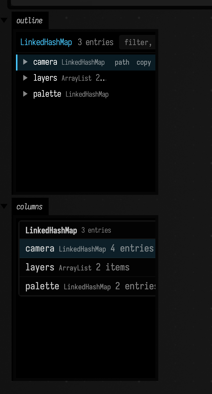
tree("channel", value)gives you an outline / tree browser.column("channel", value)gives you a column-style browser.
These are especially good for nested maps, scene graphs, structured JSON-like data, or anything you want to poke around in rather than summarize.
Both take any value, not only maps and lists. A data class or one of your own classes opens to its public properties, an IntArray or DoubleArray opens to its elements, and a map whose keys are objects opens each entry to its key and its value. Every row shows its name, its type and a one-line summary (5000 items, "label", Point(x=1.0, y=2.5, label=p)), so you can read most of a structure without opening anything:
data class Particle(val position: Vec3, val age: Double, val tag: String)
class Node(val name: String) {
    var next: Node? = null
}

val ring = Node("a")
ring.next = Node("b").also { it.next = ring }

val scene = linkedMapOf(
    "particle" to Particle(Vec3(1f, 2f, 0.5f), 0.25, "spark"),
    "weights" to doubleArrayOf(0.1, 0.4, 0.5),
    "many" to List(5000) { it * it },
    "ring" to ring,
)
tree("scene", scene)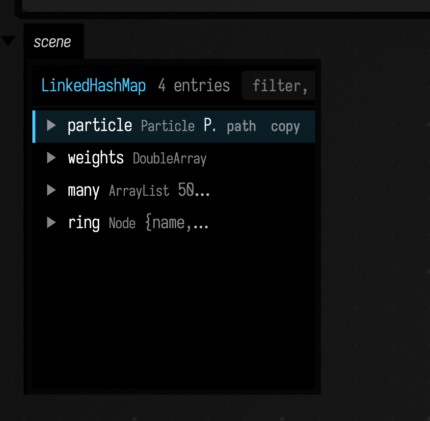
A long collection arrives 200 rows at a time; the last row says how many there are and loads the next 200. Open rows follow the value: if code that keeps running (a frames { } loop, say) adds to particles, the tree shows the new size within about a second, without re-running the box. An object that contains itself is marked with ↺ instead of being opened forever.
Keys, once you have clicked into the embed: the arrow keys move and open (in column, ← and → move between columns), / filters the rows, c copies the selected value as text, p copies the row's path, and r reloads. The header stays put while the rows scroll. The embed grows with its content up to a height and then scrolls; pass maxHeight = 800 to tree or column to change that height.
The rows are the same edges graphPaths walks, so every row has a path from the value you passed in, such as particle/position or many/250. Press p (or the path button on a row) and paste it into box code:
:::static
val age = scene.graphPath("particle/age")?.get()
Type a pattern containing /, * or | into the filter and it runs graphPaths on the whole value instead of filtering one level: **/tag lists every tag at any depth, labelled by path. Choose one (Enter, or double-click) and the tree or columns open to it. Plain text still just filters the rows in view.
This recording types **/name into the filter of a tree over a small scene of groups and layers. Every name at any depth is listed by its path; the arrow keys pick groups/1/layers/1/name, and Enter opens the tree down to it.
Private properties are left out, as graphPaths leaves them out by default. Pass includePrivate = true to tree or column to list them; their paths then need graphPaths(pattern, GraphWalkOptions(includePrivate = true)). A row has no path when nothing reaches it by name: an element of a primitive array, a map key that is an object, the second of two map keys that print alike.
Browsing the renderer
A box beneath a renderer box can open the renderer itself. It answers "what am I drawing, in what order, and where does the frame time go?" without a debugger:
column("renderer", renderer, width = 1100)renderer is already in scope beneath the renderer box. width gives the panel room for several columns side by side, and open = "render/modules" opens the columns down to that path when the browser loads (the path button on a row copies its path). The renderer opens to:
render: the window's render target. Its children are listed in the order the target records them each frame:preTargets(render-to-texture passes drawn first),modules(one permoduleHere, in the order they were added),meshModules, thenothers.- A module opens to its
parameters(name, colour attachments and format, depth, primitive type, blend), itsuniformsand texture bindings with their set and binding numbers, and itsmesheswith vertex, triangle and instance counts. compute: the compute target and its modules, drawn before graphics.cpu: the CPU spans of the frame loop (acquire, record, submit, present), with p1 to p99 times in milliseconds.windows,contexts,queues,device: the swapchain, its format and size, and the Vulkan objects behind them.
Every node with children starts with a summary row: choose it to see that node's card. The renderer's card has the frame number, module counts, the window and the p50/p90 of each CPU span. Cards follow the running renderer, refreshing about once a second. tree("renderer", renderer) shows the same nodes as an outline.
Here the column browser is open on a running renderer that draws one triangle, down to the triangle's module and its card:

Browsing a glTF scene
A scene file opens the same way. GltfSupport.loadModel gives Assimp's own view of a glTF (or any
file Assimp reads), and column(...) or tree(...) lists its root node with its transform and
children, then its meshes, materials and animations. A GltfModel loaded for drawing browses as its
meshes, each with its buffers, material, texture slots and transform.
import afield.graphics.scene.GltfSupport

val scene = GltfSupport.loadModel("dev_docs/agents/fixtures/path_tracing/transforms.gltf")!!
column("columns", scene, width = 1300)
tree("tree", scene, width = 700)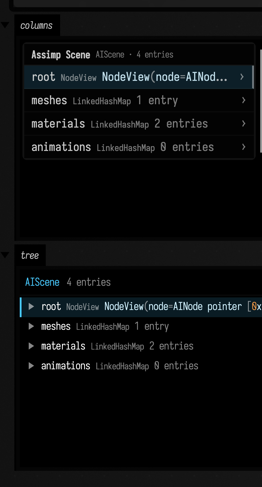
For a live log in an output panel, use logs(...). This box shows the demo channel and logs a
small job into it; rows with the same block ID are grouped under the block's first line:
logs("logs") { channel("demo") }

val log = afield.ai.diagnostics.LogDispatcher
log.log(
    afield.ai.diagnostics.LogEvent(
        "demo",
        "starting a job",
        blockId = "job",
        boundary = afield.ai.diagnostics.BlockBoundary.BEGIN,
    ),
)
for (i in 1..3) log.log(afield.ai.diagnostics.LogEvent("demo", "step $i of 3", blockId = "job"))
log.log(
    afield.ai.diagnostics.LogEvent("demo", "done", blockId = "job", boundary = afield.ai.diagnostics.BlockBoundary.END),
)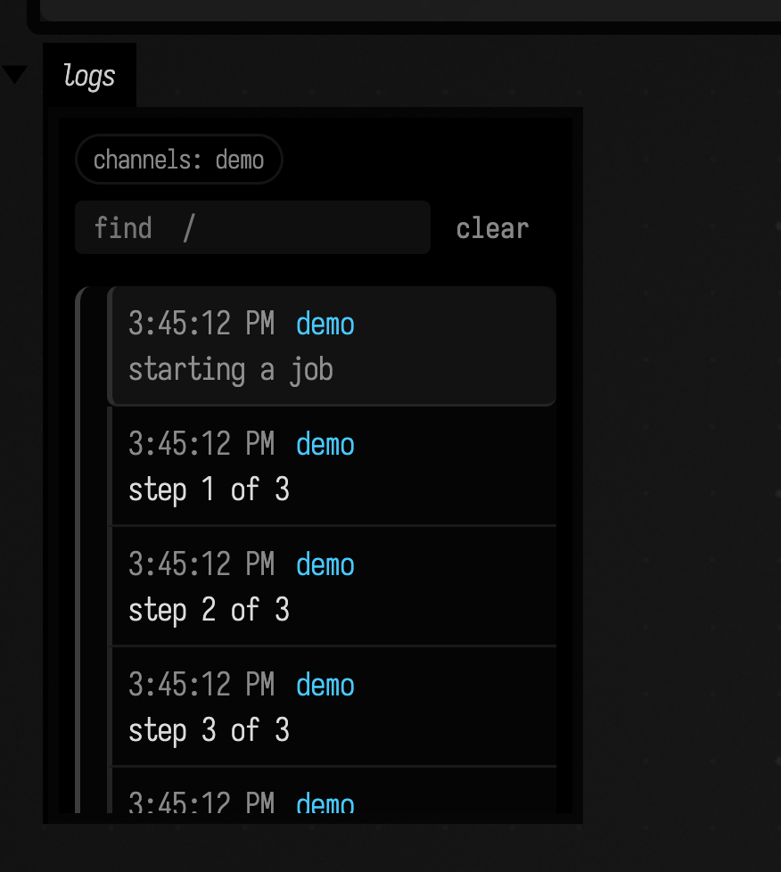
The log updates as the job runs.
The embed has a find box (/) that hides rows not containing its text, a clear button (or k), and, when you have scrolled up to read something, a ↓ N new button instead of jumping away from what you were reading. If Field restarts, the embed reconnects by itself.
Keeping output areas tidy
You can manage channels directly:
:::static
displayOpen("preview")
displayClear("preview")
displayClearAll()
This is useful for demos, guided tutorials, and boxes that are meant to be rerun frequently.
displayClear removes the panel rather than emptying it; Box Output covers all
four calls and the mouse gestures that do the same.
Controls: sliders, toggles, colors, text, and XY pads
Field can build small control surfaces directly into output areas: sliders and pads you drag while the box runs.
They also reach a phone. Open /controllers?file=<document> on it and the Group tab redraws the selected box's controlGroup(...) at thumb size, while Outputs shows its output areas with their controls still live. See Field from your phone.
:::static
controlGroup("controls") {
    slider("gain", min = 0.0, max = 1.0, step = 0.01, initialValue = 0.35) {}
    vec2Control("orbit", initialValue = Vector2f(0.35f, -0.2f)) {}
    checkbox("armed", initialValue = true) {}
    stringInput("name", initialValue = "Field") {}
    colorPicker("accent", initialValue = Vector4f(0.95f, 0.45f, 0.15f, 0.85f)) {}
}

println("controls ready")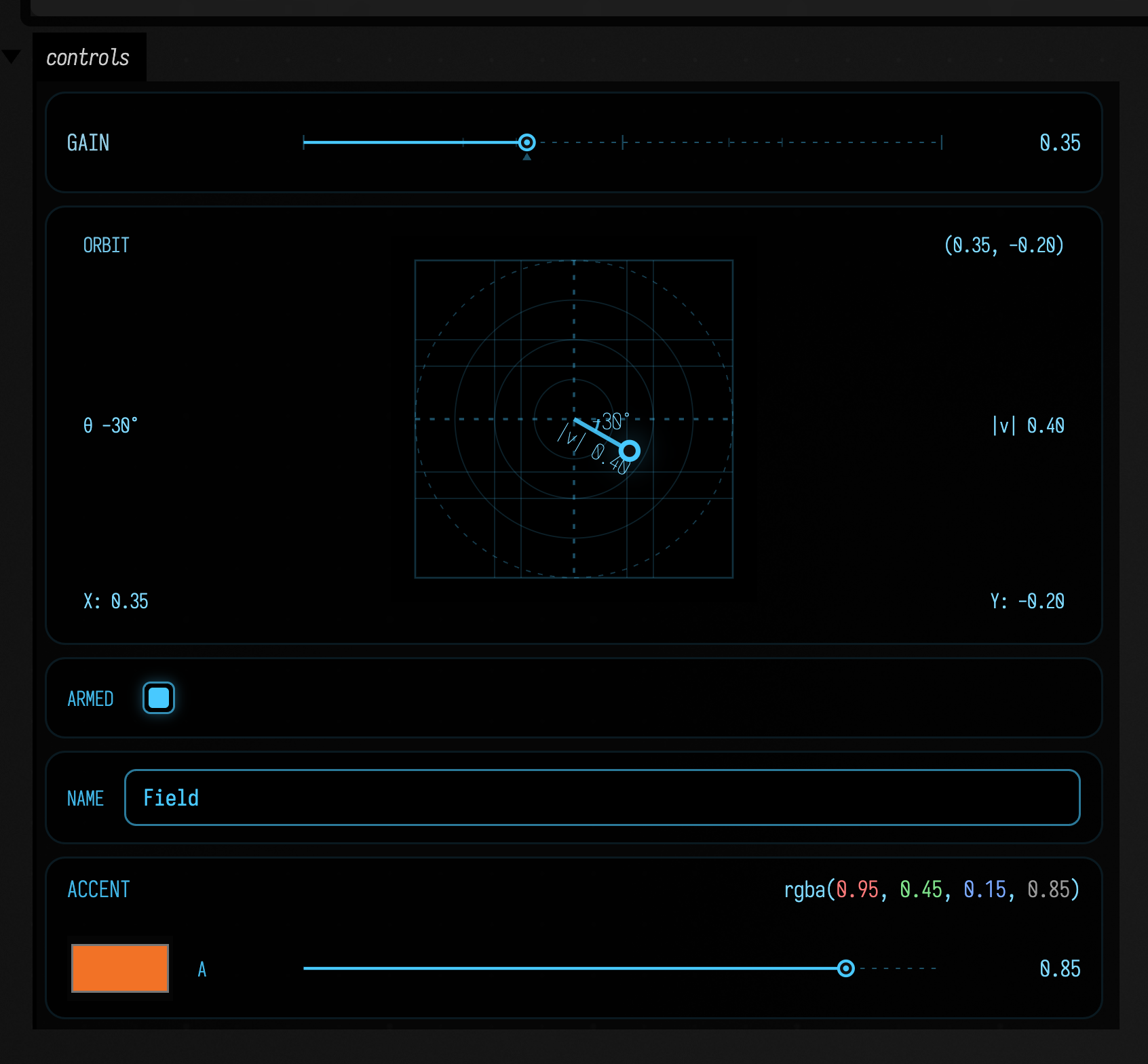
Available pieces include:
slider(...)sliders(...)vec2Control(...)checkbox(...)stringInput(...)colorPicker(...)controlGroup(...) { ... }
vec2Control(...) gives you an XY pad with a vector line and readouts for its length and angle.
Handling a slider
Standalone sliders, sliders(...) and sliders in a controlGroup share the same gestures:
This recording drags a live controlGroup slider, nudges it with the arrow key, then double-clicks
the track to return to its starting value. The large bar is updated by the slider's callback, so it
shows the value Field receives while the pointer moves.
| Do this | To get |
|---|---|
| press and drag | the thumb jumps to the pointer and follows it |
| hold shift while dragging | a relative drag, ten times finer, from wherever the value already is; pressing shift mid-drag does not make the thumb leap |
| double-click the track | the slider's initialValue again |
| click the number | type an exact value; Enter keeps it, Esc abandons it |
| arrow keys (after a click) | one step per press; shift ×10, alt ÷10. A law = slider moves 1% of its travel instead |
| PageUp / PageDown, Home / End | 10% of travel, or the ends |
| Backspace | back to initialValue |
| the mouse wheel (after a click) | one arrow press per notch, with the same shift and alt. A slider you have not clicked lets the wheel scroll the canvas |
If the box re-renders the control while you are dragging it, because its callback rebuilt the
controlGroup or the box re-ran, the drag carries on with the new control.
Handling an XY pad
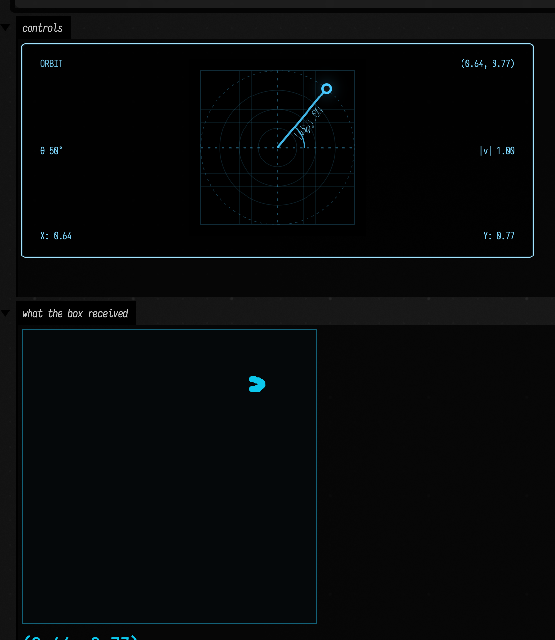
A vec2Control takes the slider's gestures in two dimensions. This recording presses the pad to put
the handle under the pointer, walks it left with the arrow keys, then holds shift and drags: the
handle moves a tenth as far as the pointer, from where it was. The dots in the panel below are each
value the callback received.
| Do this on a pad | To get |
|---|---|
| press and drag | the handle jumps to the pointer and follows it |
| hold shift while dragging | a relative drag, ten times finer, from where the handle already is |
| double-click the pad | its initialValue again |
| arrow keys (after a click) | one step along that axis, up is +y; shift ×10 |
| Backspace | back to initialValue |
| Enter | type (x, y) |
The other controls' readouts take typing too. On a vec2Control, click X or Y to set one coordinate, the (x, y) pair to set both, |v| to change the length and keep the direction, or θ (degrees) to turn it and keep the length. On a colorPicker, click the rgba(...) readout and type four numbers from 0 to 1, or a #rrggbb hex colour; click the alpha number to type the alpha alone. Typed values are clamped and snapped like a drag.
The track carries guides: ticks at the quarters, thirds and middle of its travel (the ends and middle drawn taller), a small notch under the initialValue that double-click returns to, and a mark at zero when the range runs from negative to positive. On a law = slider the ticks sit at fractions of the travel, not of the value. The vec2Control pad has the same quarter and third gridlines, plus rings around the centre at a quarter, half, three quarters and the full half-width of the pad, so a vector's length reads at a glance.
A typed or nudged value is snapped to step and clamped to the range, the same as a drag, so the callback never sees a number the slider could not have produced.
A controlGroup slider keeps its value across re-runs and in the saved document. A standalone slider(...) starts from initialValue every run. When the value should belong to the box, bind it to a property:
prop<Double>(gain)
syncToProperty("gain", 0.5, min = 0.0, max = 2.0)
syncToProperty starts from the property's current value when it has one, so re-running the box keeps whatever you last dialled in, and the property is saved with the document.
Declare the property with propDown<Double>(gain) and moving the slider also reruns every box that reads gain; see Properties that re-run boxes.
Build one surface with mixed control types
controlGroup(...) is the easiest way to build a compact surface for one box. Pair it with a normal display channel when the controls need a readable status or preview panel.
:::static
var wind = Vector2f(-0.45f, 0.30f)
var bloom = 0.62
var trails = true
var label = "wake field"
var tint = Vector4f(0.25f, 0.75f, 1.0f, 0.9f)

// Refresh after each edit. TINT controls monochrome luminance and alpha.
fun updatePreview() {
    val gray = (255 * (0.2126 * tint.x + 0.7152 * tint.y + 0.0722 * tint.z)).toInt().coerceIn(0, 255)
    val x = 160 + wind.x * 120
    val y = 48 - wind.y * 32
    val radius = 6 + bloom * 22
    val dash = if (trails) "4 3" else "none"
    markdown(
        "preview",
        """
        #### ${label.md}

        <svg width="320" height="96" viewBox="0 0 320 96" style="background:#080808;border:1px solid #555">
          <circle cx="$x" cy="$y" r="$radius" fill="rgb($gray,$gray,$gray)" fill-opacity="${tint.w}"
                  stroke="#ddd" stroke-dasharray="$dash"/>
        </svg>

        wind=(${wind.x}, ${wind.y}) · bloom=$bloom · trails=$trails
        tint=(${tint.x}, ${tint.y}, ${tint.z}, ${tint.w})
        """,
        width = 620,
    )
}

controlGroup("surface") {
    slider("bloom", min = 0.0, max = 1.0, step = 0.01, initialValue = bloom) {
        bloom = it
        updatePreview()
    }
    vec2Control("wind", initialValue = wind, xRange = -1.0 to 1.0, yRange = -1.0 to 1.0, step = 0.05) {
        wind = it
        updatePreview()
    }
    checkbox("trails", initialValue = trails) {
        trails = it
        updatePreview()
    }
    stringInput("label", initialValue = label) {
        label = it
        updatePreview()
    }
    colorPicker("tint", initialValue = tint) {
        tint = it
        updatePreview()
    }
}
// Cached controls may invoke callbacks during setup; draw once more after all are restored.
updatePreview()

println("mixed controls ready")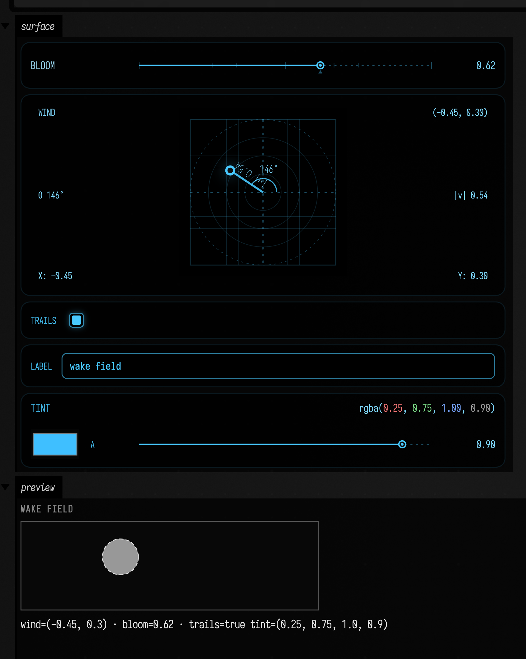
This pattern is good for surfaces that combine parameter editing with a compact readout:
- small simulation controls
- animation parameters
- quick scene presets
- reusable demo boxes
Sequencer controls: multisliders, grids, ranges and menus
These controls take their names and ideas from Max objects:
multiSlider(...)is a bank of bars you draw by sweeping across them, like Max'smultislider. A fast sweep fills every bar it passes.matrix(...)is a grid of cells, likematrixctrl. A press advances a cell to its next state, and dragging paints that state across every cell you cross. Cells are on or off by default; passstates = 4and each cell cycles through 0 to 3. State 0 is black and the others are equally spaced colours.rangeSlider(...)picks an interval, likerslider. Drag a thumb to move one end, or drag between the thumbs to move both.menu(...)picks one of a list of strings, likeumenu.
The first three return a handle with a playhead: a position the box writes and you only see. It never calls your callback and is never saved, so you can set it on every frame. Here a loop reads the step off the clock each frame, so it never drifts:
:::static
var velocity = 16 { i -> 0.5 + 0.4 * Math.sin(i * 0.6) }
var pattern = 4 { r -> 16 { c -> if ((c + r * 3) % 8 == 0) 1 + (c / 4) % 3 else 0 } }
var band = 200.0..900.0
var wave = "saw"

lateinit var steps: ArrayControlHandle<List<Double>>
lateinit var grid: ArrayControlHandle<List<List<Int>>>
lateinit var range: ArrayControlHandle<ClosedFloatingPointRange<Double>>

controlGroup("sequencer") {
    steps = multiSlider("velocity", count = 16, initialValues = velocity) { velocity = it }
    grid = matrix("pattern", rows = 4, columns = 16, states = 4, initialValue = pattern) {
        pattern = it
        print(it.h)
    }
    range = rangeSlider("band", min = 20.0, max = 2000.0, initialValue = band) {
        band = it
        print(it.h)
    }
    menu("wave", ["sine", "saw", "square", "noise"], initialIndex = 1) { _, name ->
        wave = name
    }
}

// Eight steps a second, read off the clock every frame.
val start = System.nanoTime()
loop {
    val step = ((System.nanoTime() - start) / 125_000_000L).toInt()
    steps.playhead(step % 16)
    grid.playhead(step % 16)
    range.playhead(20.0 + (step % 64) / 63.0 * 1980.0)
}
A playhead on a multislider or matrix is a bar or column index, and a negative one hides it. On a range slider it is a value on the track.
The same controls, on a dial
Pass polar = true to draw any of the three around a circle. A step sequence is a loop, and the dial shows that: the last step sits next to the first.
- On a polar
multiSlider, the angle picks the bar and the distance from the centre sets its value. A sweep across the top goes the short way round. - On a polar
matrix, rows are rings (row 0 is the outermost) and columns are sectors running clockwise from twelve o'clock. The playhead lights a whole sector. - On a polar
rangeSlider, the track is the whole circle, andminandmaxmeet at the top. The band runs clockwise fromstarttoendInclusiveand may wrap through the top. Drag inside it to turn the whole band.
On a dial a range means an arc, and value in band follows it. Use it for values that are already circular: a phase, a hue, a window into a loop.
:::static
var velocity = 16 { i -> 0.5 + 0.4 * Math.sin(i * 0.6) }
var pattern = 4 { r -> 16 { c -> if ((c + r * 3) % 8 == 0) 1 + (c / 4) % 3 else 0 } }
var band = 1700.0..400.0 // wraps through the top

lateinit var steps: ArrayControlHandle<List<Double>>
lateinit var grid: ArrayControlHandle<List<List<Int>>>
lateinit var range: ArrayControlHandle<ClosedFloatingPointRange<Double>>

controlGroup("dial", columns = 3) {
    steps = multiSlider("velocity", count = 16, initialValues = velocity, polar = true) { velocity = it }
    grid = matrix("pattern", rows = 4, columns = 16, states = 4, initialValue = pattern, polar = true) { pattern = it }
    range = rangeSlider("band", min = 20.0, max = 2000.0, initialValue = band, polar = true) {
        band = it
        print(100.0 in it)
    }
}

val start = System.nanoTime()
loop {
    val step = ((System.nanoTime() - start) / 125_000_000L).toInt()
    steps.playhead(step % 16)
    grid.playhead(step % 16)
    range.playhead(20.0 + (step % 64) / 63.0 * 1980.0)
}
Recording a gesture
gesture(...) is an XY pad that remembers what you did with it. A plain drag works like vec2Control(...), and the callback gets each position. Shift-drag records a take: the whole stroke and its timing, kept with the box like any other control value. On a phone, tap rec, then draw. The trail of the take stays on the pad.
The box controls playback. at(seconds) returns the position at a given time in the loop,
interpolating between recorded samples; playhead(seconds) shows that position on the pad. Read
both from the clock in a loop and playback continues even with the browser closed. initialTake
gives the pad something to play before you record: here it is a figure eight:
:::static
var p = Vector2f(0f, 0f)
lateinit var pad: GestureHandle

// A figure eight to start from; shift-drag on the pad to record your own.
val eight = 64 { i ->
    val a = i / 63.0 * 2 * Math.PI
    i / 63.0 * 2.0 to Vector2f((0.8 * Math.sin(a)).toFloat(), (0.6 * Math.sin(2 * a)).toFloat())
}

controlGroup("gesture") {
    pad = gesture("move", initialTake = eight) { p = it }
}

val start = System.nanoTime()
loop {
    val t = (System.nanoTime() - start) / 1e9
    pad.at(t)?.let { p = it }
    pad.playhead(t)
}
p follows your finger while you drag and the take otherwise. Use it for anything with two axes: a camera, a pan and a filter, a point in a preset space.
To edit a take key by key, bake it into keyframe lanes with bakeGesture(pad), and send the edited lanes back with pad.setTake(x, y): see From a performed gesture.
Recording a slider into keyframes
A gesture records an XY pad take, kept on the pad, which you bake into keyframes afterwards with bakeGesture. recordToggle records a single control straight into a keyframe curve. In the presets example below, recordToggle("size") adds a rec size button. Press it, move the size slider, and press it again: what you played becomes a keyframe curve named size, opened under the panel. The take is thinned to the keys needed to stay within half a percent of the slider's range, so a three-second up-down-up sweep of 62 slider changes comes back as 35 keys you can edit, not one per mouse event.
To play the curve back into the slider, read it in a loop and hand it to playControl:
val take = keyframes(name = "size")
val start = System.nanoTime()
loop {
    val t = ((System.nanoTime() - start) / 1e9) % 2.0
    take.setTime(t)
    playControl("size", take, t, channel = "look")
}
playControl moves the slider and runs its callback, so the playback drives whatever the slider drives. recordControl(label, channel) is the same recording without the button: it returns a recording whose stop() writes the curve.
Presets and morphing
presetBar(keys) adds a preset bar over a KeyframeScope: a preset is a keyframer key. Declare the values as delegated locals (var size by keys.slider(0.4, 0.1..1.0)) and add them to the group with keys.controls(), as in One value shared by a local, a control and a key. Here two keys, calm and storm, are saved the first time the box runs, so there is something to morph between straight away:
:::static
val keys = KeyframeScope()
var size by keys.slider(0.4, 0.1..1.0)
var offset by keys.vec2(Vector2f(0f, 0f))
var tint by keys.color(Vector4f(0.2f, 0.6f, 1f, 1f))
var ring by keys.checkbox(false)

fun draw() {
    val r = (20 + size * 60).toInt()
    val cx = 110 + (offset.x * 60).toInt()
    val cy = 90 - (offset.y * 50).toInt()
    val fill = "rgba(${(tint.x * 255).toInt()},${(tint.y * 255).toInt()},${(tint.z * 255).toInt()},${tint.w})"
    val stroke = if (ring) "stroke='white' stroke-width='6'" else ""
    display("main", "<svg width='220' height='180' style='background:#222'><circle cx='$cx' cy='$cy' r='$r' fill='$fill' $stroke/></svg>")
}
keys.onChange { draw() }

val dir = presetDirectory("look")

// Two keys to start from, written once; after that the stored ones are used.
if (keys.savedKeyNames(dir).isEmpty()) {
    keys.Key("size" to 0.25, "offset" to Vector2f(-0.5f, 0.3f), "tint" to Vector4f(0.2f, 0.6f, 1f, 1f), "ring" to 0f)
        .save(dir.resolve("calm"))
    keys.Key("size" to 0.95, "offset" to Vector2f(0.6f, -0.4f), "tint" to Vector4f(1f, 0.25f, 0.1f, 1f), "ring" to 1f)
        .save(dir.resolve("storm"))
}

controlGroup("look") {
    keys.controls()
    presetBar(keys)
    recordToggle("size")
    midiLearnButton()
}

draw()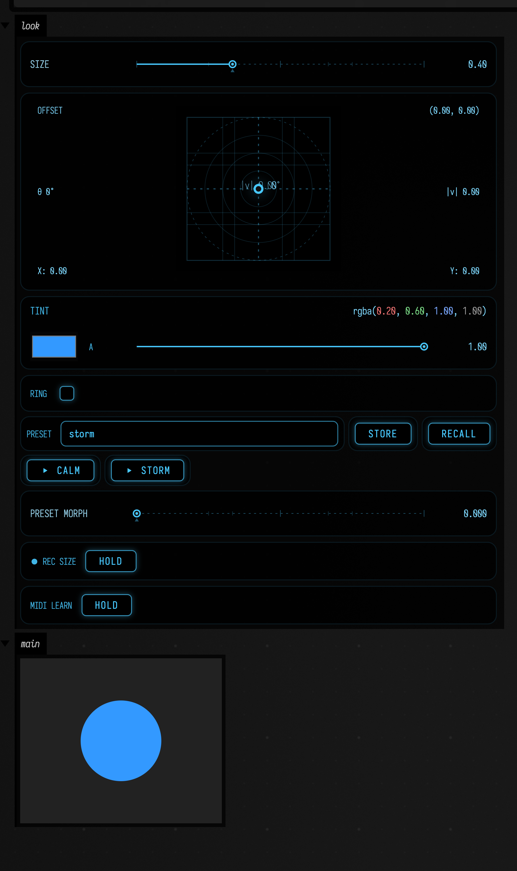
store saves the panel as a key under the name in the field. recall, or a key's own button, applies it: the locals change, the controls move and onChange runs. preset morph blends across the saved keys in name order. With calm and storm, the morph at 0.5 gives a mid-size purple circle with the ring on. presetBar returns the bar, whose store(name), recall(name) and morph(t, between) do the same from code.
The presets are ordinary key files in presetDirectory("look"). For their history, browsing and how each kind of value blends, see Saving: every save is history, Browsing saved keys and What a scope watches.
MIDI learn
midiLearnButton() adds a MIDI learn button. Press it, touch the control you want, and turn a knob on your controller (or turn the knob first, then touch the control). From then on that knob moves that control. A knob follows the control's own response, so on a logarithmic frequency slider the middle of the knob is the middle of the slider, not 10 kHz. A knob bound to a checkbox switches it on above halfway. Learning a knob that is already bound moves the binding, and the bindings are saved with the box.
midiLearn(channel) does the same from code. bind attaches a knob by its controller number, attach listens to a MIDI input, and feed hands it a controller value from anywhere else — a test, an OSC message, or the loop below, which stands in for a knob:
var cutoff = 1000.0
var bright = false
controlGroup("synth") {
    slider("cutoff", 20.0, 20000.0, initialValue = cutoff, law = ControlLaw.LOGARITHMIC) { cutoff = it }
    checkbox("bright", bright) { bright = it }
    midiLearnButton()
}
val midi = midiLearn("synth")
midi.bind("cutoff", cc = 74)
midi.bind("bright", cc = 64)
// What a knob sends; with hardware, midi.attach(MidiDevices.openInput(MidiDevices.inputs().first())).
for (v in [0, 32, 64, 96, 127]) {
    midi.feed(0, 74, v)
    println("CC74 = $v  ->  cutoff ${cutoff.f1}")
}
midi.feed(0, 64, 127)
midi.feed(0, 74, 80)
println("bright = $bright, bindings = ${midi.bindings}")
It prints the cutoff at 20, 114, 650, 3705 and 20000 as the stand-in knob goes from 0 to 127: the middle of the knob lands near the middle of the log scale.
To hear hardware, open an input with MidiDevices and attach it: midi.attach(MidiDevices.openInput(MidiDevices.inputs().first())), or pass the input to midiLearnButton(input).
Choosing the right control
- Use
slider(...)for one bounded numeric value. - Use
vec2Control(...)for direction, position, velocity, or any paired numeric parameter. - Use
checkbox(...)for feature toggles and gates. - Use
stringInput(...)for names, labels, prompts, and small text parameters. - Use
colorPicker(...)for RGBA values stored as normalizedVector4fdata. - Use
multiSlider(...)for a row of values you want to draw rather than set one at a time: steps, envelopes, partials. - Use
matrix(...)for patterns: on/off steps, or several states per cell withstates = n. - Use
rangeSlider(...)for an interval, such as a band, a window or a velocity range. Usepolar = truewhen the value wraps around, like a phase or a hue. - Use
menu(...)for choosing one of a few named options. - Use
gesture(...)for a two-axis movement you want to perform once and loop. - Use
recordToggle(...)to perform one control's movement into a keyframe curve, andpresetBar(keys)to store and morph between whole settings of a panel. - For a curve over time you shape by hand, an envelope, use the keyframe editor,
keyframes(...): see Keyframes and timelines.
The vec2Control(...) includes an XY pad, a vector line, and magnitude readout, so it works well for motion and layout values where two sliders would hide the relationship between axes.
Recorded audio: waveform, player, playhead, and navigation
AudioVisualizer is the general-purpose recorded-sound view. It combines a waveform and native
browser audio controls, keeps an optional vertical playhead synchronized with playback, and uses
the waveform itself as a navigator:
- click to seek;
- drag to pan;
- use the mouse wheel or
+/−to zoom while keeping the visible playhead fixed on screen; - shift-wheel to pan;
- double-click or press all to restore the complete clip.
If the playhead is outside the visible interval, wheel zoom falls back to the pointer and button or
keyboard zoom falls back to the center. Near the start or end of a recording, boundary clamping may
move the playhead on screen. A completion-style spinner remains over the waveform while a newly
zoomed or panned min/max envelope is loading, so the old waveform cannot be mistaken for the new
view. During playback, crossing the right edge advances the visible interval and places the playhead
slightly inside the new window; crossing the left edge after a backward seek mirrors that behavior.
Set followPlayhead = false in AudioVisualizerOptions to keep a zoomed interval stationary.
Waveform-envelope requests have a 15-second browser deadline; a stalled service clears the spinner
and reports a timeout instead of leaving the view permanently busy. Any subsequent pan, zoom, or
resize retries normally.
Short sample arrays can be embedded in the page. This example opens zoomed in, with the playhead parked inside the visible window.
:::static
val sampleRate = 8_000
val seconds = 5.0
val recording =
    FloatArray((sampleRate * seconds).toInt()) { i ->
        val t = i / sampleRate.toDouble()
        val chirp = sin(2.0 * PI * (105.0 * t + 72.0 * t * t))
        val low = 0.34 * sin(2.0 * PI * 47.0 * t)
        val pulse = if ((t * 2.0).toInt() % 2 == 0) 0.16 * exp(-8.0 * (t % 0.5)) else 0.0
        (0.54 * chirp + low + pulse).toFloat()
    }

displayAudioSamples(
    samples = recording,
    sampleRate = sampleRate,
    options = AudioVisualizerOptions(
        width = 1050,
        waveformHeight = 150,
        showPlayhead = true,
        initialStartSeconds = 0.8,
        initialDurationSeconds = 2.7,
        initialPositionSeconds = 1.45,
    ),
    label = "five-second synthetic recording",
)

println("recorded audio visualizer ready")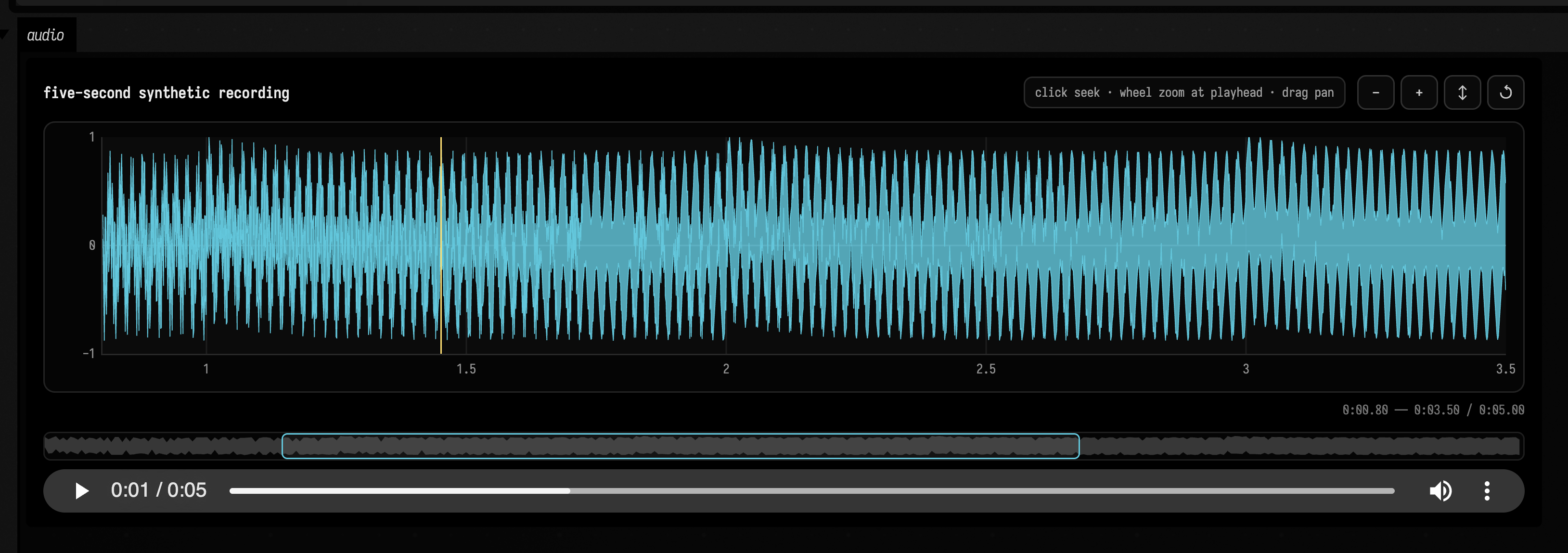
There are three general entry points from a Field box:
// A browser-accessible recording. Add waveformUrl for range-aware server summaries.
displayAudio(
    AudioVisualizerSource(
        audioUrl = "/recordings/long-take.wav",
        waveformUrl = "/analysis/long-take/waveform",
        durationSeconds = 183.4,
        label = "long take",
    ),
)

// Generated or transformed mono samples; encoded as a self-contained PCM16 WAV.
displayAudioSamples(samples, sampleRate = 48_000, label = "synthesis result")

// Short existing recordings. Long files should use URLs instead of inflating box output.
displayAudioBytes(mp3Bytes, mediaType = "audio/mpeg", label = "short field recording")
All three return the generated HTML as well as displaying it, so it can be composed into a larger
instrument panel. AudioVisualizer.renderHtml(...), renderSamplesHtml(...), and
renderBytesHtml(...) are the receiver-free forms when no implicit Field box is available.
For a Field Audio service representation, use the same component without transferring or decoding the complete recording just to draw it:
val representation: AssetRepresentation = candidate.proxyRepresentation!!
display(
    "audio",
    representation.audioVisualizerHtml(
        options = AudioVisualizerOptions(showPlayhead = true),
    ),
)
That adapter asks the service for a bounded min/max envelope of only the visible interval. Each
source frame contributes to a pixel's minimum or maximum, preserving short transients that simple
sample decimation would miss. Zooming and panning request a new envelope with at most 4096 points;
the audio itself continues to stream from the immutable representation. Set showPlayhead = false
for a waveform-only inspection surface.
Shared time cursors and transport
Audio players and arbitrary time-based views can share a loose, browser-side timeline. Give them
the same syncGroup. A component whose local zero is later on the source timeline also gets an
offset; shared time is always localSeconds + syncOffsetSeconds.
val group = "nancy-analysis"

display(
    "source",
    representation.audioVisualizerHtml(
        options = AudioVisualizerOptions(
            initialStartSeconds = 18.0,
            initialDurationSeconds = 24.0,
            initialPositionSeconds = 18.0,
            syncGroup = group,
        ),
    ),
)

// Analysis-local 0 s corresponds to source 18 s.
display(
    "analysis",
    analysisDashboardHtml(
        [beats, mono, poly],
        syncGroup = group,
        timeOffsetSeconds = 18.0,
    ),
)
The two players below share syncGroup = "two-players"; the second holds the source from 1 s, so it is given syncOffsetSeconds = 1.0. Pressing play on the first moves both playheads, a second apart in local time:
This synchronizes across separate display(...) output documents. Playback publishes a gold
playhead to every joined view; hover publishes a temporary cursor; click publishes a seek; and zoom
or pan publishes a visible time window. The callback protocol is small, and is also available
to handwritten HTML, gesture views and future timeline widgets through parent-window
CustomEvents:
const bus = window.parent === window ? window : window.parent

bus.addEventListener("field-time-cursor", event => {
    const { group, time, kind, active } = event.detail
    // kind is "hover" or "playhead"
})

bus.dispatchEvent(new bus.CustomEvent("field-time-seek", {
    detail: { group: "nancy-analysis", source: "my-view", time: 23.75 }
}))
field-time-window carries {group, source, start, duration} and field-time-transport reports
play / pause. Receivers ignore their own source, so callbacks can adapt or republish events
without a feedback loop.
One viewer for functions, sounds and signals
Fn.plot, the audio player, displaySignal and the analysis views are the same component. They
differ in where the data comes from: samples embedded in the page, an audio envelope, or a
server query per visible window. Give them one syncGroup and they share a timeline. Zoom one
and the others follow, hover shows a cursor in all three, and a click in any of them seeks the
audio.
:::static
// One viewer, three sources, one timeline: a decaying 220 Hz ping.
val sync = "one-viewer"
val rate = 8_000
val ping = { t: Double -> sin(2 * PI * 220 * t) * exp(-2.5 * t) }

// 1. Fn.plot: the envelope, samples embedded in the page (resampled live when you zoom in).
with(Functions) {
    val envelope = fn(0.0..2.0, "envelope  exp(-2.5 t)") { t -> exp(-2.5 * t) }
    envelope.plot("envelope", syncGroup = sync, xLabel = "seconds")
}

// 2. displayAudioSamples: the ping itself, playable; click to seek.
displayAudioSamples(
    FloatArray(2 * rate) { ping(it / rate.toDouble()).toFloat() },
    rate,
    channel = "audio",
    label = "the ping, as audio",
    options = AudioVisualizerOptions(width = 760, syncGroup = sync),
)

// 3. displaySignal: the same ping evaluated per visible window on the server.
displaySignal(
    SignalViewer([SignalChannel("ping", ping, -1.0, 1.0)], 0.0, 2.0, sampleStep = 1.0 / rate),
    "signal",
    SignalViewerOptions(
        width = 760,
        label = "the ping, evaluated per window",
        syncGroup = sync,
        viewKey = "one-viewer:signal",
    ),
)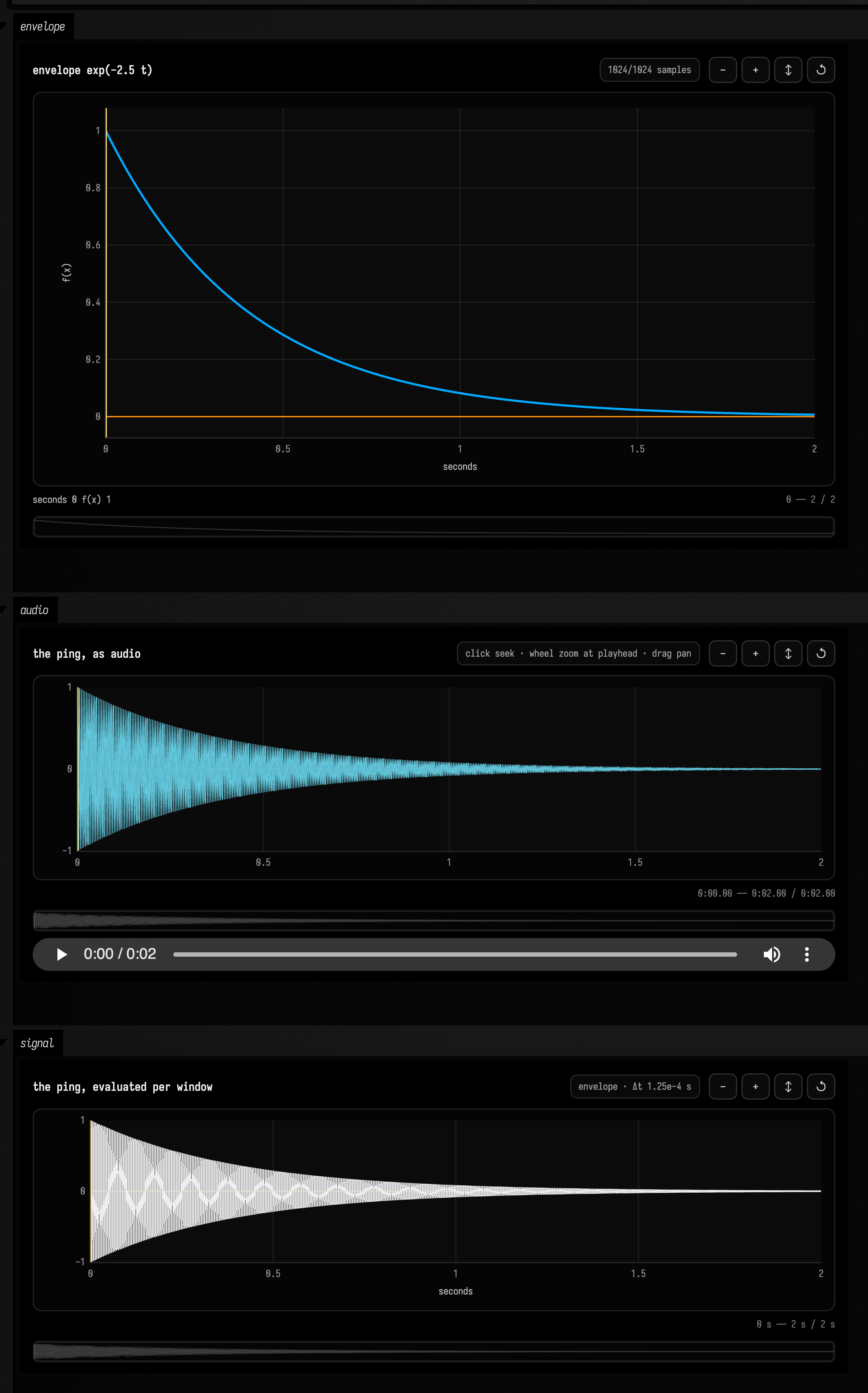
The chip in each header says what you are looking at. For the function it is 1024/1024 samples
until you zoom inside the domain, and then live · Δx …, because Fn.plot resamples the function
as you zoom. For the signal it is the sampling grid, envelope · Δt … or waveform · Δt …. The
strip under each plot is the whole domain. It stays dim until you zoom, then marks the visible
window; click or drag it to move. The ripple in the white band is the signal's sampling grid
showing through: at this zoom each bin holds about ten samples, roughly a third of a 220 Hz cycle,
so a bin's min and max rarely land on a peak. Zoom in and it becomes the waveform.
Beat and pitch analysis views
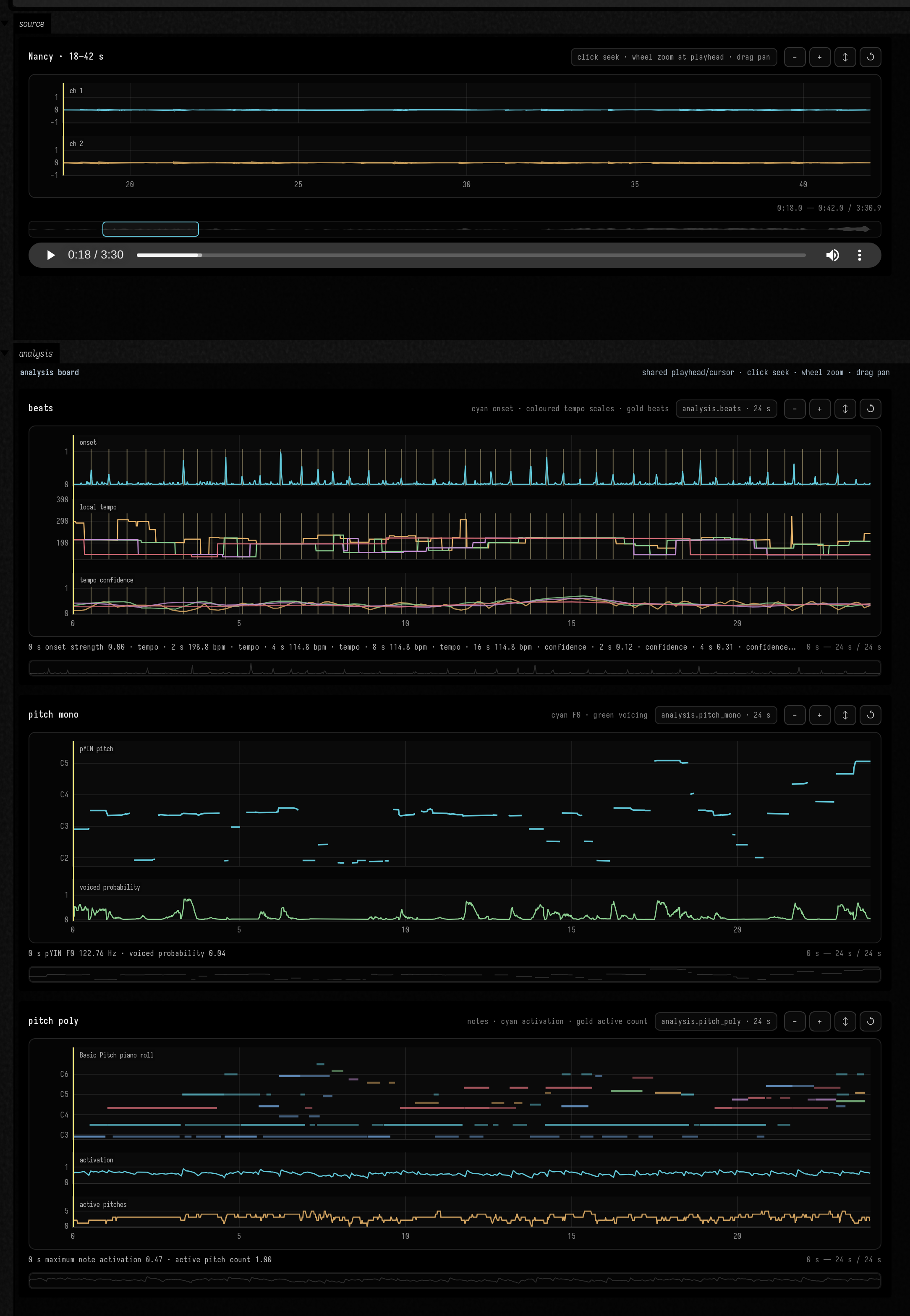
Field Audio can show beat and pitch analyses alongside a recording. The full results stay in NPZ
files, while analysisVisualizationHtml(...) draws previews on a timeline you can zoom and pan:
- multi-scale tempo curves, onset strength, and beat markers;
- monophonic pYIN pitch and voicing confidence;
- Basic Pitch polyphonic note rectangles and activity summaries.
The beat and pitch analysis walkthrough runs all three jobs on a recording and draws the board.
val client = FieldAudioClient()
client
    .assetByFilename("*Nancy*")
    .thenCompose { asset ->
        val region = AssetRegion(asset.id, startSeconds = 0.0, durationSeconds = 30.0)
        client.submit(multiScaleBeatAnalysis(region, scalesSeconds = [2.0, 4.0, 8.0, 16.0]))
    }
    .thenCompose(client::awaitAnalysis)
    .thenAccept { result ->
        display("analysis", analysisVisualizationHtml(result))
    }
Replace the request with monophonicPitchAnalysis(region) or
polyphonicPitchAnalysis(region) without changing the job/result path. The returned
AnalysisResult exposes the complete NPZ representation and, for Basic Pitch, a MIDI artifact.
The visualization endpoint caps previews at 4096 points; zoom and pan never turn the full activation
tensor into a large JSON response.
To compare results, analysisDashboardHtml(listOf(beats, mono, poly)) lines them up and keeps
zoom, pan, hover and playback together. If you already have an AnalysisPreview, use
analysisPreviewVisualizationHtml(...) or analysisPreviewDashboardHtml(...) to show it without
fetching again. For progress, fieldAudioJobStatusHtml(accepted, event) displays one job and
fieldAudioJobMonitor() shows the queue.
The beat and pitch analysis walkthrough and loadable
audio_ai_analysis operation transcript contain the full source → submit → monitor → await →
visualize path.
Speech embedding phase portraits
The emotion2vec and WavLM views from the speech walkthrough:
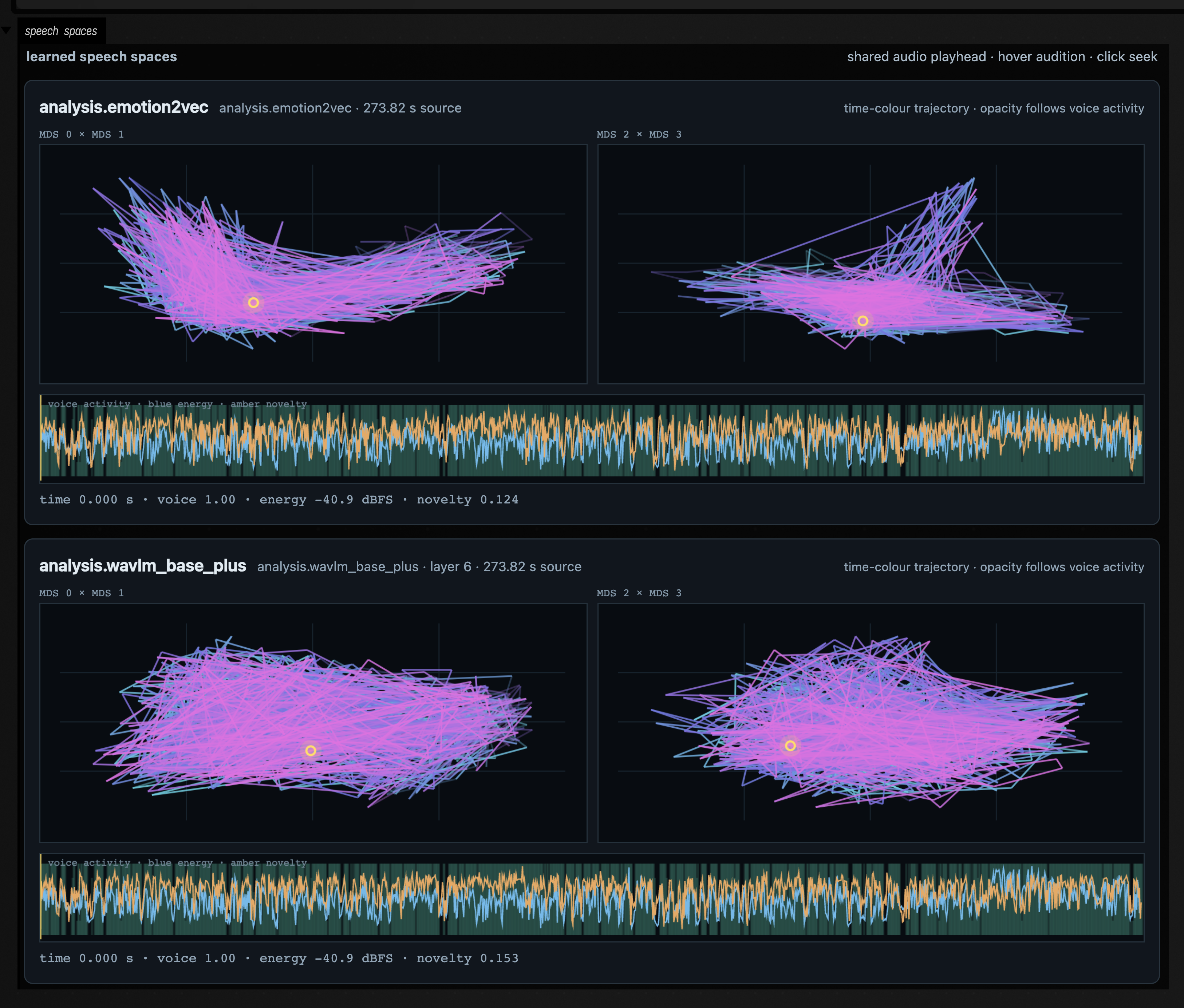
speechEmbeddingVisualizationHtml(result) turns the worker's cached learned-frame preview into two phase
portraits: MDS axes 0×1 and 2×3. The complete 768-dimensional embedding remains in the immutable
NPZ; only a bounded preview crosses into the browser. A strip underneath shows WebRTC voice
activity, dBFS energy, and embedding novelty.
Give the source AudioVisualizer and the speech view the same syncGroup. Audio playback moves a
marker through both portraits; hovering either portrait publishes the nearest frame time; clicking
seeks the player. The view also listens to field-time-window, so the waveform's visible interval
stays saturated while the rest of the embedding path recedes. These are the same general
field-time-cursor, field-time-seek, and field-time-window callbacks used by the timeline
analysis views.
val sync = "field-recording-speech"
display(
    "source",
    audio.audioVisualizerHtml(
        options = AudioVisualizerOptions(syncGroup = sync),
    ),
)

client.submit(wavlmBasePlusEmbeddingAnalysis(region, layer = 6)).thenCompose(client::awaitAnalysis).thenAccept { result
    ->
    display("WavLM", speechEmbeddingVisualizationHtml(result, syncGroup = sync))
}
Use speechEmbeddingDashboardHtml(listOf(emotion2vec, wavlm), syncGroup = sync) to compare both
models on one playhead. speechEmbeddingPreviewVisualizationHtml(...) and
speechEmbeddingPreviewDashboardHtml(...) are the no-fetch counterparts. The complete
speech-reactive embedding walkthrough and
audio_ai_speech_embeddings transcript show import → submit → monitor → await → audition.
For a programmable local-neighbourhood projection, prefer
client.speechEmbeddingSmileTsnePreview(result, poolMillis = 500.0, hopMillis = 40.0). It downloads
the result's binary MessagePack tensor, selects the requested time range before float16 expansion,
mean-pools 500 ms of evidence around each point, and runs fixed-seed t-SNE inside Field using Smile.
The independent 40 ms hop produces 25 points per second, just above a 24 fps display. Both values
round to the model's native 20 ms grid; omit them to retain the original 50 Hz vectors. Pooling occurs
before maxFrames sampling, and the visualizer header reports the effective pool, hop, distance, and
projected frame count. The returned AnalysisPreview goes directly into the no-fetch visualizers.
Exact classical MDS remains available through
speechEmbeddingSmilePreview; both paths support cosine and Euclidean distance without rerunning
the neural analysis.
Short-time spectral phase portraits
Three distance spaces from the spectral walkthrough:
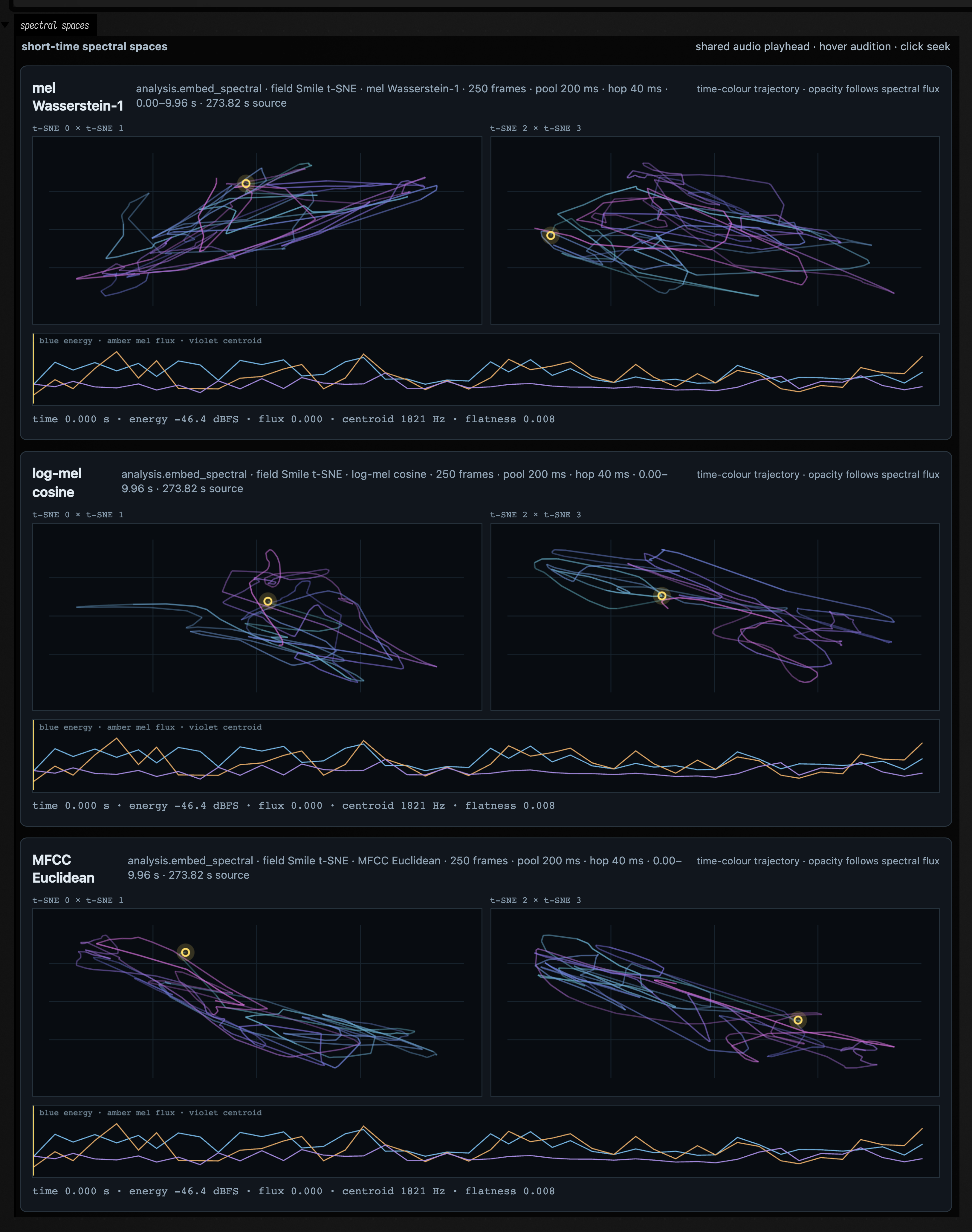
spectralEmbeddingPreviewVisualizationHtml(preview) uses the same two phase portraits and shared
time bus for a Field-owned MDS or t-SNE projection of mel, log-mel, or MFCC frames. The lower strip
shows energy, mel-distribution flux, and spectral centroid; path opacity follows normalized flux.
Hovering reports time, energy, flux, centroid, and flatness, and clicking seeks any linked audio
visualizer.
One analysis.embed_spectral result contains all three representations, so decode once and create
several views without another job:
client
    .analysisPreview(result.id)
    .thenCombineAsync(
        client.spectralEmbeddingFrames(
            result,
            durationSeconds = 10.0,
            poolMillis = 200.0,
            hopMillis = 40.0,
        ),
    ) { preview, frames ->
        [
            SpectralEmbeddingDistance.MEL_WASSERSTEIN,
            SpectralEmbeddingDistance.LOG_MEL_COSINE,
            SpectralEmbeddingDistance.MFCC_EUCLIDEAN,
        ].map { distance ->
            preview.withSpectralProjection(frames.tsne(distance = distance, dimensions = 4))
        }
    }
    .thenAccept { previews ->
        display("spaces", spectralEmbeddingPreviewDashboardHtml(previews, syncGroup = "recording"))
    }
The short-time spectral walkthrough takes a recording through analysis and projection into all three spaces, then lets you listen while exploring them.
Instrument-labelled transcription
A recording and its recovered notes from the MuScriptor walkthrough:
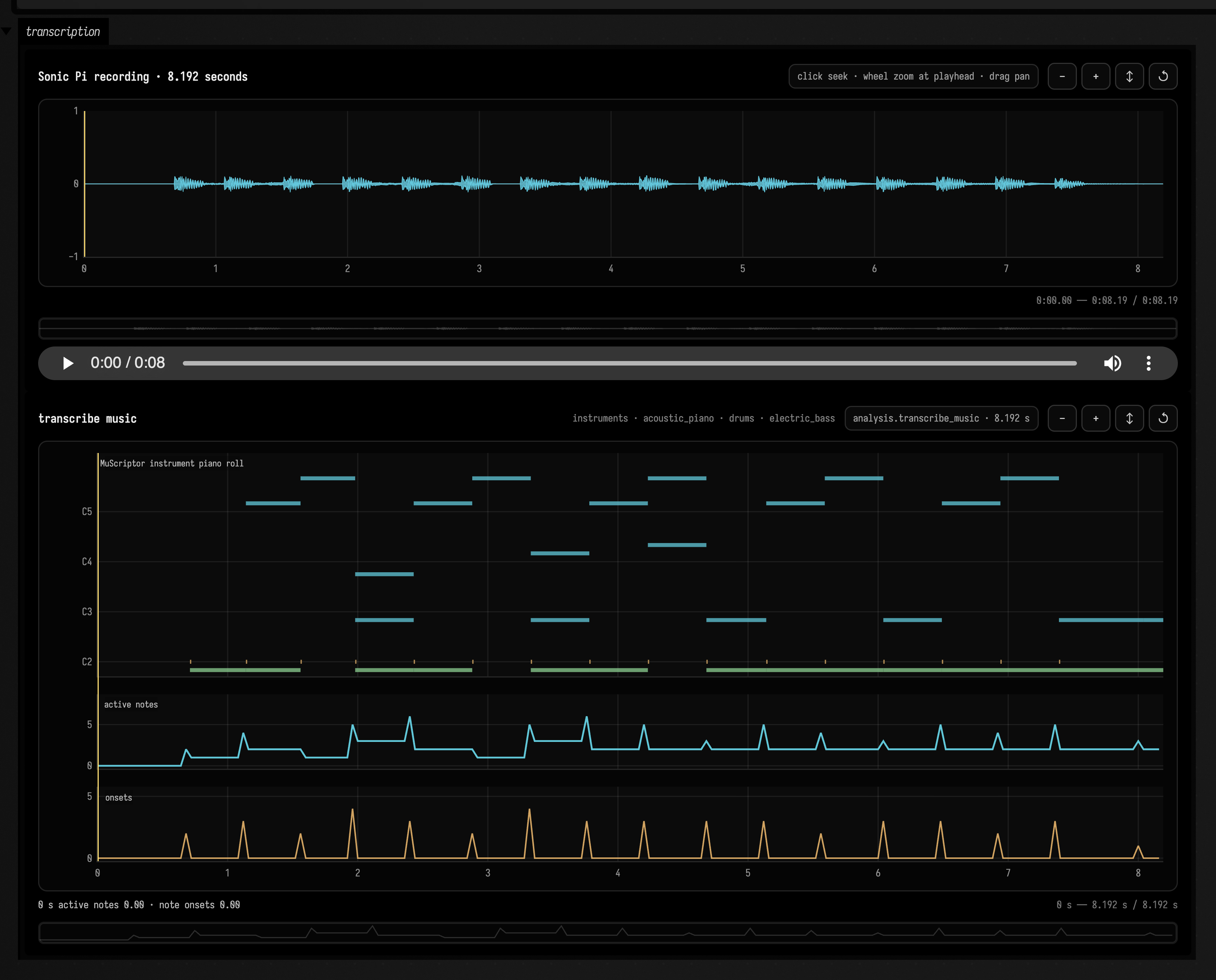
The same analysisVisualizationHtml viewer recognizes analysis.transcribe_music results as a
MuScriptor piano roll. Note colour follows the recovered instrument group; the two lower lanes show
active polyphony and onset count. It uses the same syncGroup time bus as the waveform, beat,
pitch, speech-space, and spectral-space views, so playback, hover, seek, zoom, and pan stay aligned.
val sync = "recording-to-score"
display(
    "source",
    audio.audioVisualizerHtml(
        options = AudioVisualizerOptions(syncGroup = sync),
    ),
)
display(
    "score",
    analysisVisualizationHtml(
        transcription,
        syncGroup = sync,
    ),
)
The MuScriptor walkthrough follows a recording through transcription, the synchronized display and MIDI export.
The same visualizer can begin with sound generated inside Field. renderPatWav, renderDirtWav,
renderDoughWav, renderFaustWavAsync, and recordSonicPiWav all produce a
RenderedAudioFile; client.analyzeRenderedAudio(render) imports it and returns a
RenderedAudioAnalysis whose visualizationHtml() joins the playable waveform and every analysis
lane on one sync group. The render-to-analysis walkthrough and
audio_render_analysis transcript show all five paths through submission and progress monitoring.
Corpus neighbour microscope
Retrieved neighbour windows from the corpus walkthrough:
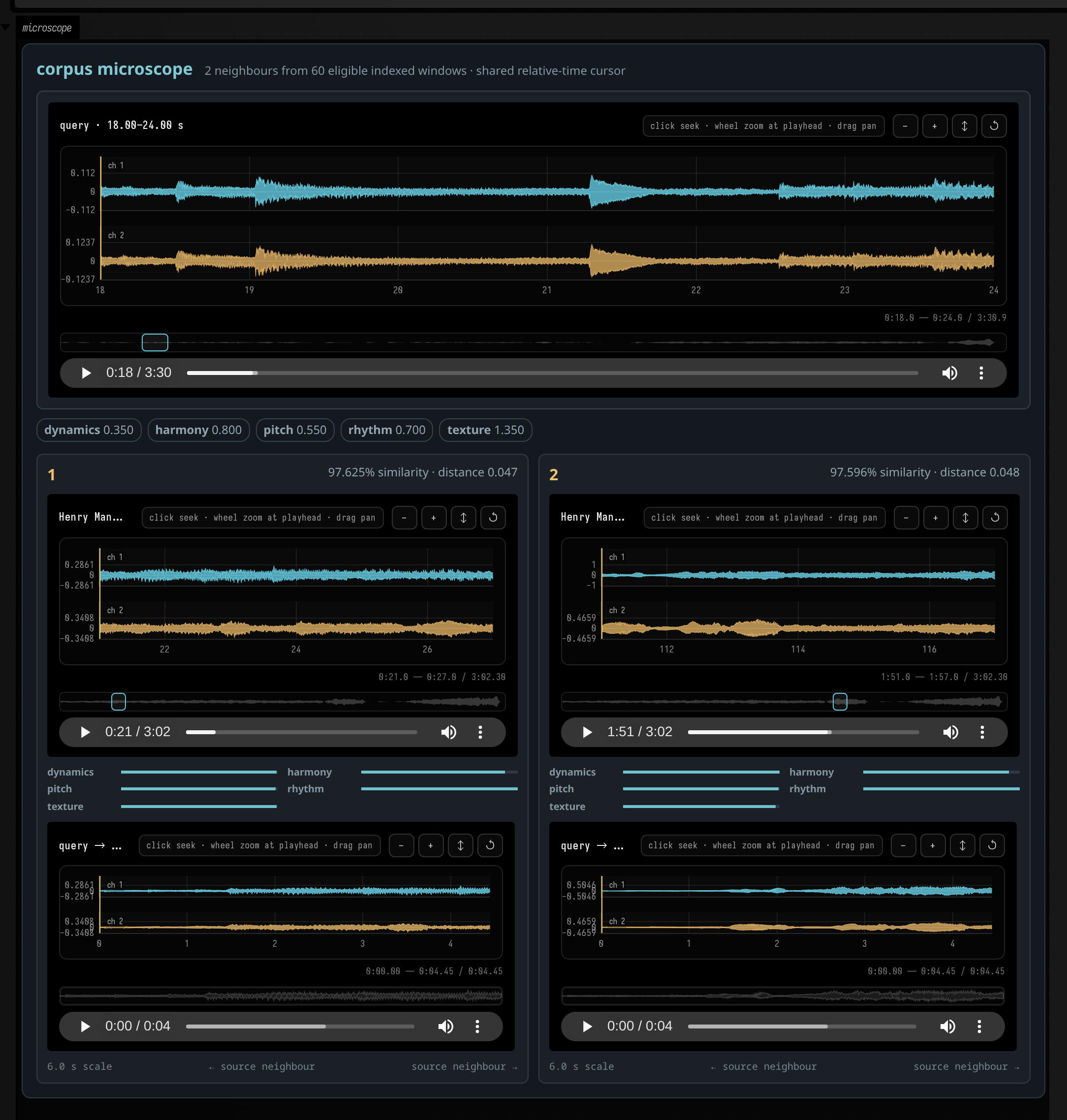
corpusMicroscopeHtml(preview, queryAudio) composes the same general AudioVisualizer into a
source-relative A/B board. Each neighbour retains its real asset and source timestamp, but every
player uses syncOffsetSeconds = -segment.startSeconds; shared time zero is therefore the start of
the selected window even when two windows come from different recordings. Hover, zoom, seek and
playhead callbacks remain ordinary field-time-* events.
The board adds no waveform transport of its own. It supplies exact ranges, grouped distance bars,
and the immutable query-to-neighbour splice preview returned by Field Audio. That makes it useful as
a general pattern for comparing aligned excerpts: produce a CorpusPreview, choose the query WAV
representation, and let the range-aware player request only the visible envelopes.
The corpus microscope walkthrough shows how to index a collection and compare a passage with its neighbours.
Waveform-summary endpoint contract
This player fetches its envelopes from the live Field Audio waveform endpoint.
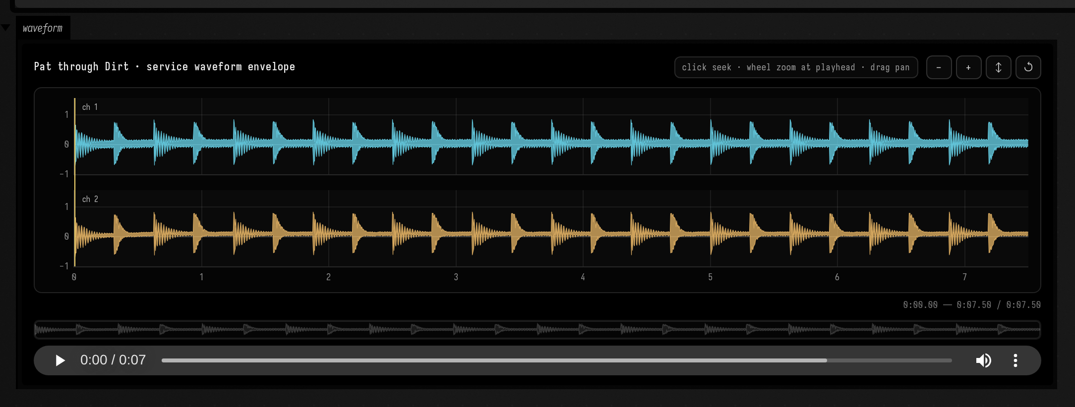
AudioVisualizer is not coupled to Field Audio. Any HTTP service can provide waveformUrl. The
visualizer adds these query parameters whenever its visible interval changes:
start_seconds=12.5&duration_seconds=4.0&points=960The endpoint returns one min/max envelope per channel:
{
  "start_seconds": 12.5,
  "duration_seconds": 4.0,
  "sample_rate": 48000,
  "channels": 2,
  "point_count": 960,
  "minimum": [[-0.4, -0.2], [-0.3, -0.1]],
  "maximum": [[0.5, 0.3], [0.4, 0.2]]
}
Each channel array must contain point_count values. The two-value arrays above are
abbreviated. Keep the response cacheable: the component aborts stale requests while
the user pans and asks for a fresh, pixel-sized envelope after zooming or resizing.
Signal and synth visualizers
Field's synth layer has HTML and SVG views for audio patches, scopes, envelopes and compressors. They appear in an output panel, with room to show more than fits beside a line of code.
:::static
val sampleRate = 48_000f
val frames = 512
val cycles = 16
val out = FloatArray(frames)

fun renderSignal(signal: Signal) {
    repeat(cycles) {
        signal.render(out, frames, SynthContext(sampleRate, frames))
    }
}

val audioScope = (saw / FreeVerb()).scope()
renderSignal(audioScope)

val monoScope = (saw / MoogLadder(cutoff = 900.p)).scope()
renderSignal(monoScope)

val g = Gate().also { it.open() }
val env = ADSR(gate = g, release = 0.4.p)
renderSignal(env)
g.close()
renderSignal(env)

val comp = Compressor(threshold = (-18).p, ratio = 6.p)
comp.input = saw * 0.35
renderSignal(comp)

println("signal visualizers ready")
display("audio", audioScope.summaryHtml(widthPx = 560, waveformHeightPx = 72, spectrumHeightPx = 72))
display("scope", monoScope.summaryHtml(widthPx = 560, waveformHeightPx = 72, spectrumHeightPx = 72))
display("env", env.stateSvg())
display("comp", comp.stateSvg())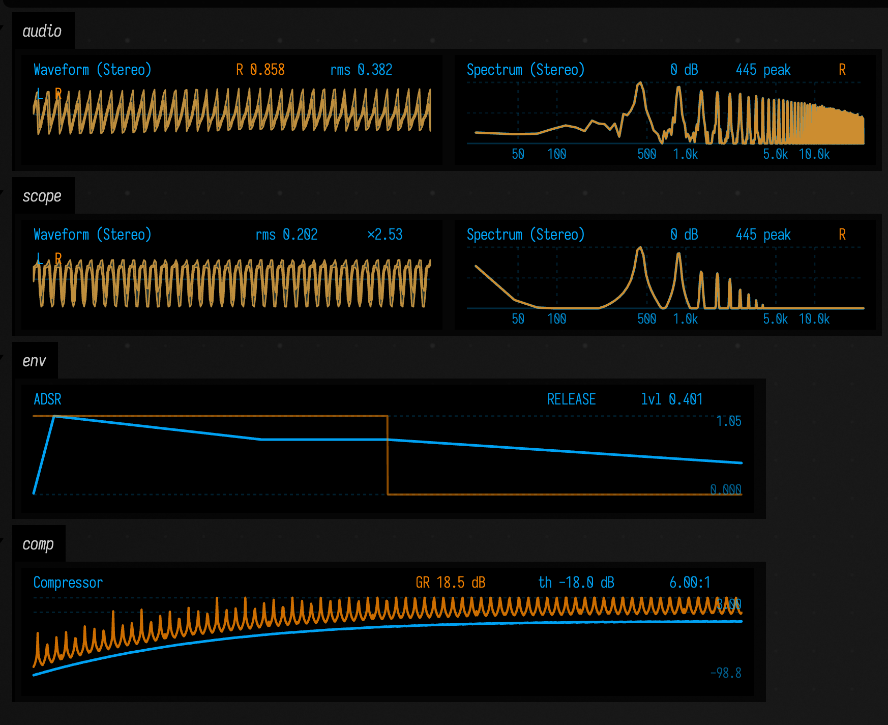
Good things to know here:
patch.summaryHtml()gives you a panel view of an audio patch.patch.liveSummary(...)andscope.liveSummary(...)keep those panels moving while audio is running.scope.summaryHtml()andstereoScope.summaryHtml()render wave/spectrum-style panels when you want a snapshot instead.env.stateSvg()andcomp.stateSvg()are compact SVG views for modulators / processors.noteProcess.pianoRollSvg()is great when you want the piano roll in an output area instead of inline in the editor.
Choose the view that gives your patch or signal enough room.
Choosing between inline and display
Here is the practical rule of thumb:
- If the visual explains one line of code, put it inline on a stack mark (ᛟ, Insert Stack Mark).
- If the visual explains a whole box or deserves interaction, put it in
display(...). - If the thing is large and structural, use
tree(...),column(...), or.h2. - If the thing is tiny and human-readable,
.his often perfect.
histogram(...) and history(...) return the value they were given, so you can leave them in a computation while you debug it.
All of these tools compose. One box can have a little inline history, a piano roll, a browser in one output channel, and a control surface in another. Field is very happy when code is also an interface.
The public declarations used on this page are listed, with their KDoc, in the codebase reference: ValueVisualizer.kt, ImagingVisualizer.kt, plotly.kt. Start from what's already in the box.