Flow Matching

flowMatch fits a velocity field to carry one cloud of points toward another. Integrating that field from t = 0 to t = 1 moves the first distribution toward the second; stopping part-way gives you an intermediate stage. The input is a few hundred to a few thousand points in two or three dimensions — a sampled FLine with noise around it is the usual case — and training takes about a second.

The method is short enough to state completely. Pick a point x0 from where you are starting and a point x1 from where you want to end up, and declare that the straight line between them is the path a particle should take: at time t it sits at \( x_t = (1-t)\,x_0 + t\,x_1 \) travelling at \( x_1 - x_0 \). Then fit a network v(x, t) to that velocity by least squares over many random (x0, x1, t) triples. No two straight lines agree where they cross, so the fit cannot reproduce any one of them; the fit seeks the average velocity through each point at each time. In the ideal case, integrating that field transports the starting distribution to the target. The loss is a regression mean squared error; the examples below show how closely a finite model gets.

:::static
val field = flowMatch(myCloud) // from a Gaussian: a generator
val fresh = field.sample(500) // new points shaped like myCloud
val threads = field.paths(80) // the trajectories, as FLines

val morph = flowMatch(to = cloudB, from = cloudA)
val halfway = morph.transport(cloudA, to = 0.5) // a real intermediate distribution

Sampling new points shaped like a cloud

With no from cloud the particles start from a standard Gaussian, which makes the result a generator: sample draws points that were not in the training data but are shaped like it.

The panels are the target cloud with the generated one on top of it, then the trajectories that produced it. Each trajectory starts somewhere in the Gaussian blur at the centre and ends on the ring.

:::static
fun cloud(points: List<Vec3>, size: Double, c: Vec4, shift: Vec3 = vec(0, 0, 0)): FLine {
    val f = FLine()
    points.forEach { f.moveTo(it + shift) }
    f.pointed = true
    f.pointSize = size
    f.color = c
    return f
}

val target = (0 until 500).map {
    val a = random() * 2 * PI
    vec(100 * cos(a), 100 * sin(a), 0.0)
}

val field = flowMatch(target, options = FlowMatchOptions(steps = 6000, seed = 11))
val samples = field.sample(500, seed = 12)

// The ring's radius is a single number, so the fit can be stated rather than eyeballed.
val radii = samples.map { hypot(it.x.toDouble(), it.y.toDouble()) }
val mean = radii.average()
val sd = sqrt(radii.sumOf { (it - mean) * (it - mean) } / radii.size)

val threads = field.paths(80, steps = 48, seed = 13).map {
    it.color = vec(0.44, 0.83, 0.78, 0.55)
    it.thickness = 0.8
    it
} + vec(330, 0, 0)
:::fold draw both panels and report the radius
lines(
    [
        // Target underneath at a larger point size, so it shows as a halo where the two agree.
        cloud(target, 3.0, vec(0.55, 0.55, 0.62, 0.9)),
        cloud(samples, 1.4, vec(0.44, 0.83, 0.78, 1.0)),
    ] + threads,
    w = 1000.0,
    h = 460.0,
    fitToSize = true,
)
markdown(
    "fit",
    """
    ~~~
generated radius   ${mean.f1} +/- ${sd.f1}   (target: 100)
chamfer to target  ${chamferDistance(samples, target).f2}
training loss      ${field.loss(200).f4} over ${field.parameterCount} parameters
    ~~~
""",
)
:::endfold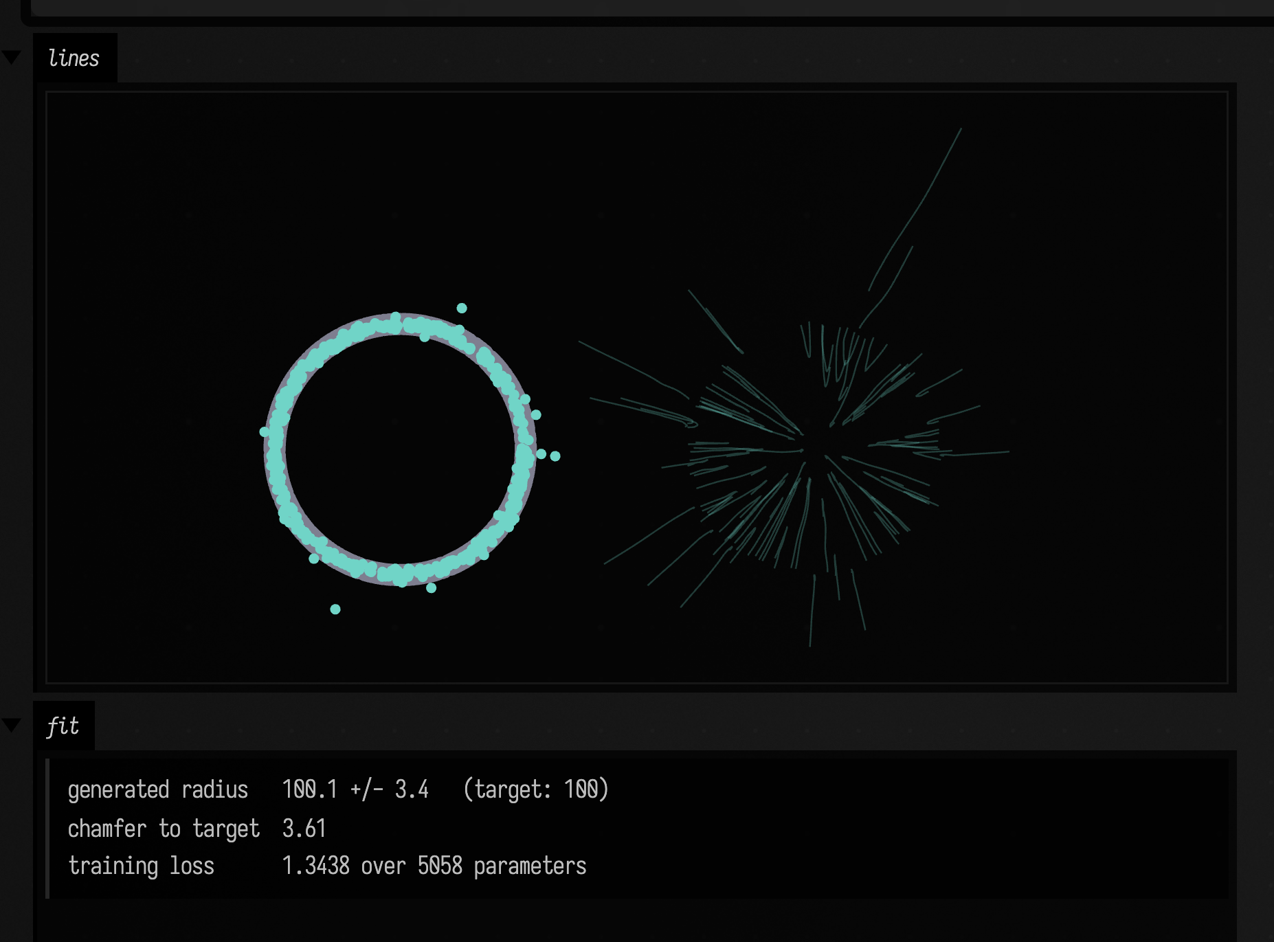

The training loss settles near 1.3 and stays there, because most of it is irreducible. Where paths cross, the field can only predict their average, and that residual is a property of the problem rather than of the fit. Loss is therefore not a quality measure here; compare samples instead, with chamferDistance or by looking.

Two conventions are chosen for you. Training happens in a centred, isotropically scaled frame, since a Gaussian source has to be commensurate with the data and FLine coordinates are usually in the hundreds; the scaling is one factor rather than one per axis, so a shape keeps its aspect ratio, and everything you pass in and get back is in your own coordinates. And 2D against 3D is decided by the data rather than by an argument: a cloud whose z never varies trains as a two-dimensional problem and its samples come back on that same plane. FlowMatchOptions.dimension overrides that.

Moving one cloud onto another

Given a from cloud the field becomes a map between two shapes, and transport can stop at any t. transport(cloudA, to = 0.5) is a genuine intermediate distribution rather than a vertex-wise average of two point lists.

When something upstream already knows which point goes where — a shared arc coordinate along two curves, say — FlowCoupling.PAIRED uses that correspondence instead of guessing one. The target velocity then becomes a function of (x, t) rather than an average over crossing paths, the loss floor drops from the data's variance to near zero, and the result can be graded point by point: this point was supposed to land there, and it landed here.

Doing that exposes a limit that matters when choosing the source shape. Integrating a velocity field is a continuous invertible map, so it can deform a curve but cannot tear a loop open or join two strands. Asking a straight segment to become a closed ring pulls the segment's two ends to the same target point, and their paths have to cross. The left panel gives the closed target a closed source; the right panel gives it a segment, at identical settings.

:::static
val n = 300

// Both curves are sampled in order of their own arc coordinate, so point i at one end is the same
// material point as point i at the other. That is what PAIRED needs.
fun closed(radius: Double): List<Vec3> = (0 until n).map {
    val s = it / (n - 1.0)
    vec(radius * cos(2 * PI * s), radius * sin(2 * PI * s), 0.0)
}

val target = closed(100.0)
val circleSource = closed(30.0)
val segmentSource = (0 until n).map { vec(200 * (it / (n - 1.0) - 0.5), -150.0, 0.0) }

val options = FlowMatchOptions(steps = 6000, seed = 11, coupling = FlowCoupling.PAIRED)
val fromCircle = flowMatch(target, circleSource, options = options)
val fromSegment = flowMatch(target, segmentSource, options = options)

fun miss(field: FlowMatchField, source: List<Vec3>): Double {
    val landed = field.transport(source, steps = 64)
    return landed.indices.sumOf { (landed[it] - target[it]).length().toDouble() } / n
}
:::fold draw the two morphs side by side and report where each point landed
fun asClosed(points: List<Vec3>, c: Vec4, t: Double): FLine = fline {
    if (points.isNotEmpty()) data("m l+", points)
    color = c
    thickness = t
}

/*
Grey is the target, purple the source at t = 0, cyan the flow between them -- the same three
roles, in the same three colours, as every other figure on this page. The target is drawn even
though the t = 1 stage lands on top of it, because otherwise there is nothing to judge against.
*/
fun stages(field: FlowMatchField, source: List<Vec3>): List<FLine> = [
    asClosed(target, vec(0.45, 0.45, 0.52, 0.9), 3.0),
    asClosed(source, vec(0.6, 0.42, 0.85, 1.0), 1.8),
] +
        [0.25, 0.5, 0.75, 1.0].map {
            asClosed(field.transport(source, to = it, steps = 48), vec(0.44, 0.83, 0.78, 0.9), 1.2)
        }

lines(
    stages(fromCircle, circleSource) + (stages(fromSegment, segmentSource) + vec(260, 0, 0)),
    w = 1000.0,
    h = 500.0,
    fitToSize = true,
)
markdown(
    "miss",
    """
    ~~~
closed source (circle -> ring)    mean landing error ${miss(fromCircle, circleSource).f2}
open source   (segment -> ring)   mean landing error ${miss(fromSegment, segmentSource).f2}
    ~~~
""",
)
:::endfold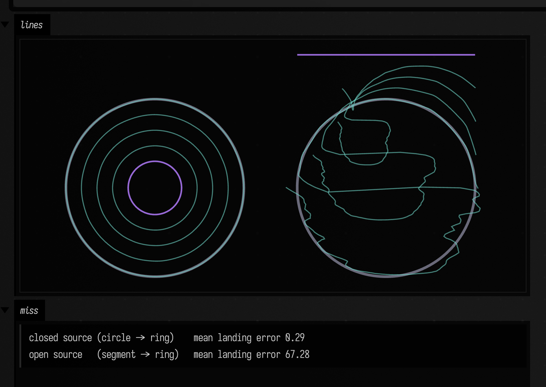

The numbers under the figure are roughly 0.3 units against 67 on a radius-100 ring. The topology mismatch costs more than every other setting on this page combined, and training longer does not help: a longer run only fits the crossing-averaged velocity more precisely. Give a closed target a closed source, an open target an open one.

FlowCoupling has a third option, MINIBATCH_OT, which pairs points within each batch by solving the assignment that minimises total squared travel. It cuts the training loss by about ten times because it removes most of the crossing. It does not follow that the samples improve: on the ring above it is slightly worse than independent pairing, since it only ever sees one batch of the cloud at a time. INDEPENDENT is the default.

Width along the curve

A centreline discards what the cloud says about its own spread. If the source strand is given a constant transverse thickness and the target tube's thickness varies along its length, the field learns both the bend and the change in width.

Here the source is a straight strand of constant width 9, and the target is a wiggling curve whose width swells from 3 at the ends to 29 in the middle. The four panels are the source and three stages of the flow.

:::static
val n = 1200

// Each sample is (s along the curve, r across it), so source and target share a point identity.
val draws: List<Pair<Double, Double>> = (0 until n).map { Pair(random(), randomGaussian()) }

fun width(s: Double): Double = 3.0 + 26.0 * sin(PI * s) * sin(PI * s)
fun centre(s: Double): Vec3 = vec(240 * (s - 0.5), 70 * sin(3 * PI * s), 0.0)

// Unit normal of the centreline: the direction the width is measured along.
fun normal(s: Double): Vec3 {
    val dy = 70.0 * 3 * PI * cos(3 * PI * s)
    val len = hypot(240.0, dy)
    return vec(-dy / len, 240.0 / len, 0.0)
}

val source = draws.map { vec(240 * (it.first - 0.5), 150 + 9 * it.second, 0.0) }
val target = draws.map { (s, r) -> centre(s) + normal(s) * (width(s) * r) }

val field = flowMatch(
    target,
    source,
    options = FlowMatchOptions(steps = 8000, seed = 11, coupling = FlowCoupling.PAIRED),
)

// Transverse spread measured along the centreline normal, so it reports width rather than a blob
// radius that would also contain the travel along the curve.
fun transverseSd(points: List<Vec3>, from: Double, to: Double): Double {
    val picked = draws.indices.filter { draws[it].first >= from && draws[it].first < to }
    val offsets = picked.map {
        val s = draws[it].first
        val d = points[it] - centre(s)
        (d.x * normal(s).x + d.y * normal(s).y).toDouble()
    }
    return sqrt(offsets.sumOf { it * it } / offsets.size)
}
:::fold draw four stages and measure the width profile against the target
fun cloud(points: List<Vec3>, c: Vec4, shift: Vec3): FLine {
    val f = FLine()
    points.forEach { f.moveTo(it + shift) }
    f.pointed = true
    f.pointSize = 1.0
    f.color = c
    return f
}

val flowed = field.transport(source, steps = 64)
lines(
    [
        cloud(source, vec(0.6, 0.42, 0.85, 0.85), vec(0, 0, 0)),
        cloud(field.transport(source, to = 0.35, steps = 48), vec(0.44, 0.83, 0.78, 0.85), vec(280, 0, 0)),
        cloud(field.transport(source, to = 0.7, steps = 48), vec(0.44, 0.83, 0.78, 0.85), vec(0, 360, 0)),
        cloud(target, vec(0.35, 0.35, 0.4, 0.7), vec(280, 360, 0)),
        cloud(flowed, vec(0.44, 0.83, 0.78, 0.85), vec(280, 360, 0)),
    ],
    w = 1000.0,
    h = 540.0,
    fitToSize = true,
)

val rows =
    (0 until 8).map { bin ->
        val lo = bin / 8.0
        val hi = (bin + 1) / 8.0
        val wanted =
            draws.indices
                .filter { draws[it].first >= lo && draws[it].first < hi }
                .map { width(draws[it].first) }
                .average()
        "  %.2f-%.2f   %7.2f   %10.2f   %10.2f"
            .format(
                lo,
                hi,
                wanted,
                transverseSd(target, lo, hi),
                transverseSd(flowed, lo, hi),
            )
    }
markdown(
    "width",
    """
    ~~~
transverse width at t = 1, measured along the centreline normal

   s band     wanted   target cloud   flowed cloud
${rows.joinToString("\n")}
    ~~~
""",
)
:::endfold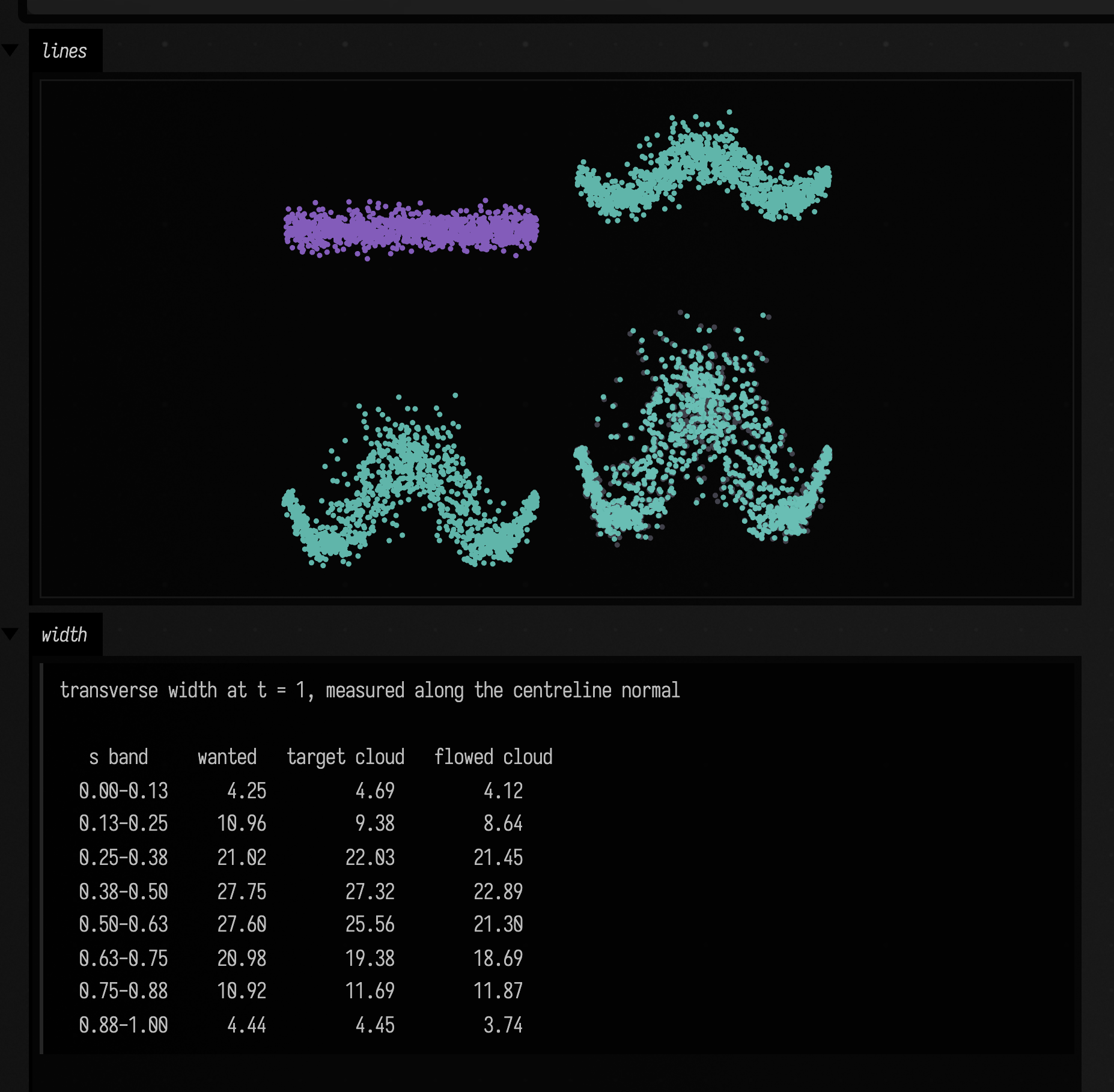

The table compares the width the target was built with, the width its own finite sample actually has, and the width the flow produced. The two agree to a few percent over most of the curve. The widest two bands come out roughly 10–17% narrow, which is where the source's constant width has to expand most.

Because the correspondence is explicit, the exact answer is known at every t, not only at the end: particle i should be at \( (1-t)\,x_{0,i} + t\,x_{1,i} \). Comparing the integrated path against that straight line measures the field directly.

:::static
val n = 1200
val draws: List<Pair<Double, Double>> = (0 until n).map { Pair(random(), randomGaussian()) }

fun width(s: Double): Double = 3.0 + 26.0 * sin(PI * s) * sin(PI * s)
fun centre(s: Double): Vec3 = vec(240 * (s - 0.5), 70 * sin(3 * PI * s), 0.0)

// Unit normal of the centreline: the direction the width is measured along.
fun normal(s: Double): Vec3 {
    val dy = 70.0 * 3 * PI * cos(3 * PI * s)
    val len = hypot(240.0, dy)
    return vec(-dy / len, 240.0 / len, 0.0)
}

val source = draws.map { vec(240 * (it.first - 0.5), 150 + 9 * it.second, 0.0) }
val target = draws.map { (s, r) -> centre(s) + normal(s) * (width(s) * r) }

val field = flowMatch(
    target,
    source,
    options = FlowMatchOptions(steps = 8000, seed = 11, coupling = FlowCoupling.PAIRED),
)

val drift =
    [0.0, 0.1, 0.25, 0.5, 0.75, 0.9, 1.0].map { t ->
        val flowed = field.transport(source, to = t, steps = 64)
        val away = (0 until n).sumOf {
            val exact = source[it] * (1 - t) + target[it] * t
            hypot((flowed[it].x - exact.x).toDouble(), (flowed[it].y - exact.y).toDouble())
        } / n
        "  %.2f   %14.2f   %10.2f%%".format(t, away, 100 * away / 240.0)
    }
:::fold draw the paths over the exact straight lines
val every = source.indices.filter { it % 16 == 0 }
val exact = every.map { i ->
    fline {
        moveTo(source[i])
        lineTo(target[i])
        color = vec(0.88, 0.64, 0.33, 0.7)
        thickness = 1.0
    }
}
val flown = field.pathsFrom(every.map { source[it] }, steps = 48).map {
    it.color = vec(0.44, 0.83, 0.78, 0.8)
    it.thickness = 0.9
    it
}

lines(exact + flown, w = 1000.0, h = 400.0, fitToSize = true)
markdown(
    "drift",
    """
    ~~~
how far the integrated path is from the exact straight line

     t   mean deviation   of a 240-unit extent
${drift.joinToString("\n")}
    ~~~
""",
)
:::endfold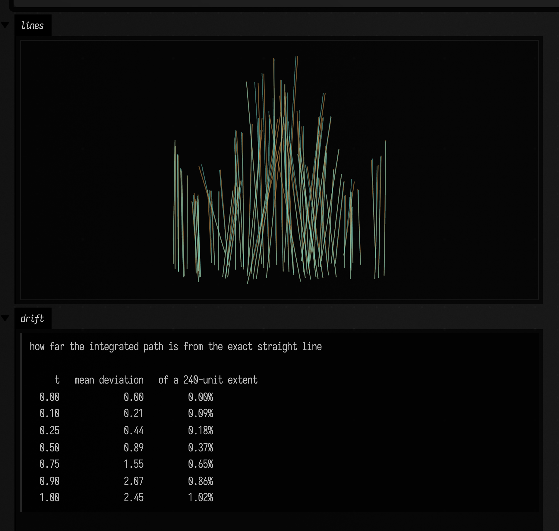

The deviation grows smoothly from zero and reaches about 1.2% of the shape's extent at t = 1. The cyan curves sit on the orange lines, which is what a paired flow looks like when the paths do not fight each other. An intermediate stage rendered on its own is correspondingly tight; several stages drawn on top of one another look much noisier than any one of them is.

Three dimensions

Nothing above is specific to the plane. A flat circle can become a trefoil knot, which is a good test because the source has no z at all and every part of the knot's depth has to be produced by the flow. Orbit the view to see it.

:::static
val n = 400

val knot = (0 until n).map {
    val u = 2 * PI * (it / (n - 1.0))
    vec(26 * (sin(u) + 2 * sin(2 * u)), 26 * (cos(u) - 2 * cos(2 * u)), -26 * sin(3 * u))
}
// A closed source for a closed target, and flat: z is entirely the field's work.
val circle = (0 until n).map {
    val u = 2 * PI * (it / (n - 1.0))
    vec(45 * cos(u), 45 * sin(u), 0.0)
}

val field = flowMatch(
    knot,
    circle,
    options = FlowMatchOptions(steps = 12000, seed = 11, coupling = FlowCoupling.PAIRED),
)
val landed = field.transport(circle, steps = 96)
val miss = circle.indices.sumOf { (landed[it] - knot[it]).length().toDouble() } / n
:::fold draw the source, the knot, and where the flow landed
fun asLine(points: List<Vec3>, c: Vec4, t: Double): FLine = fline {
    if (points.isNotEmpty()) data("m l+", points)
    close()
    color = c
    thickness = t
}

/*
Three curves only. Intermediate stages of a self-intersecting knot, overlaid in one static
projection, cannot be told apart; they are worth orbiting through live but not worth printing.
Grey target, purple source, cyan where the flow landed.
*/
threeLines(
    [
        asLine(knot, vec(0.42, 0.42, 0.5, 0.9), 4.0),
        asLine(circle, vec(0.6, 0.42, 0.85, 1.0), 2.0),
        asLine(landed, vec(0.44, 0.83, 0.78, 1.0), 1.6),
    ],
    channel = "trefoil3d",
    height = 460,
    editable = false,
)
markdown(
    "knot",
    """
    ~~~
mean landing error ${miss.f2} on a knot about 150 units across
    ~~~
""",
)
:::endfold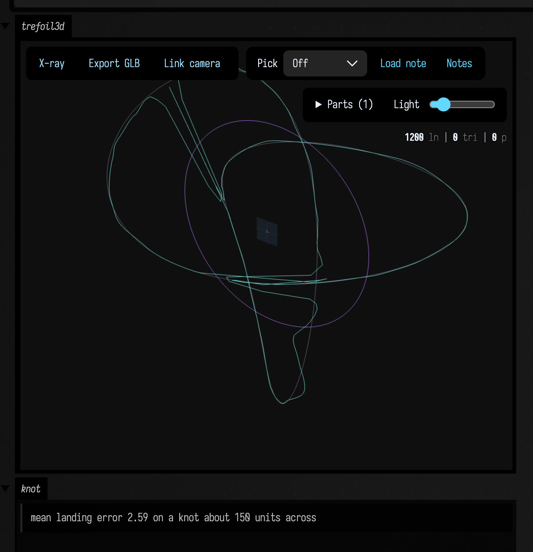

The same applies to width in three dimensions. A round canonical tube can become a helix whose cross-section both swells along its length and turns elliptical, which is the three-dimensional form of the width layer above.

:::static
val n = 1400
val picks: List<Triple<Double, Double, Double>> =
    (0 until n).map { Triple(random(), randomGaussian(), randomGaussian()) }

val source = picks.map { (s, a, b) -> vec(200 * (s - 0.5), -90 + 7 * a, 7 * b) }
val target = picks.map { (s, a, b) ->
    val u = 3 * PI * s
    val swell = 2.0 + 18.0 * sin(PI * s) * sin(PI * s)
    vec(200 * (s - 0.5) + swell * a * 0.45, 55 * sin(u) + swell * a, 55 * cos(u) + swell * 0.35 * b)
}

val field = flowMatch(
    target,
    source,
    options = FlowMatchOptions(steps = 12000, seed = 11, coupling = FlowCoupling.PAIRED),
)
val landed = field.transport(source, steps = 96)
:::fold draw the trajectories in depth
fun cloud(points: List<Vec3>, c: Vec4, size: Double): FLine {
    val f = FLine()
    points.forEach { f.moveTo(it) }
    f.pointed = true
    f.pointSize = size
    f.color = c
    return f
}

// A thinned set of threads over the two clouds, so the tube itself is visible and not only the
// travel: the round source below, the swollen helical target where the threads land.
val threads =
    field
        .pathsFrom(
            source.indices.filter { it % 28 == 0 }.map { source[it] },
            steps = 56,
        )
        .map {
            it.color = vec(0.44, 0.83, 0.78, 0.35)
            it.thickness = 0.8
            it
        }

threeLines(
    [
        cloud(source, vec(0.6, 0.42, 0.85, 0.9), 1.6),
        cloud(landed, vec(0.44, 0.83, 0.78, 0.9), 1.6),
    ] + threads,
    channel = "tube3d",
    height = 460,
    editable = false,
)
markdown(
    "miss3d",
    """
    ~~~
3D tube, ${field.dimension} dimensions inferred
mean landing error ${"%.2f".format(
    landed.indices.sumOf {
        (landed[it] - target[it]).length().toDouble()
    } / n
)} of a 200-unit extent
    ~~~
""",
)
:::endfold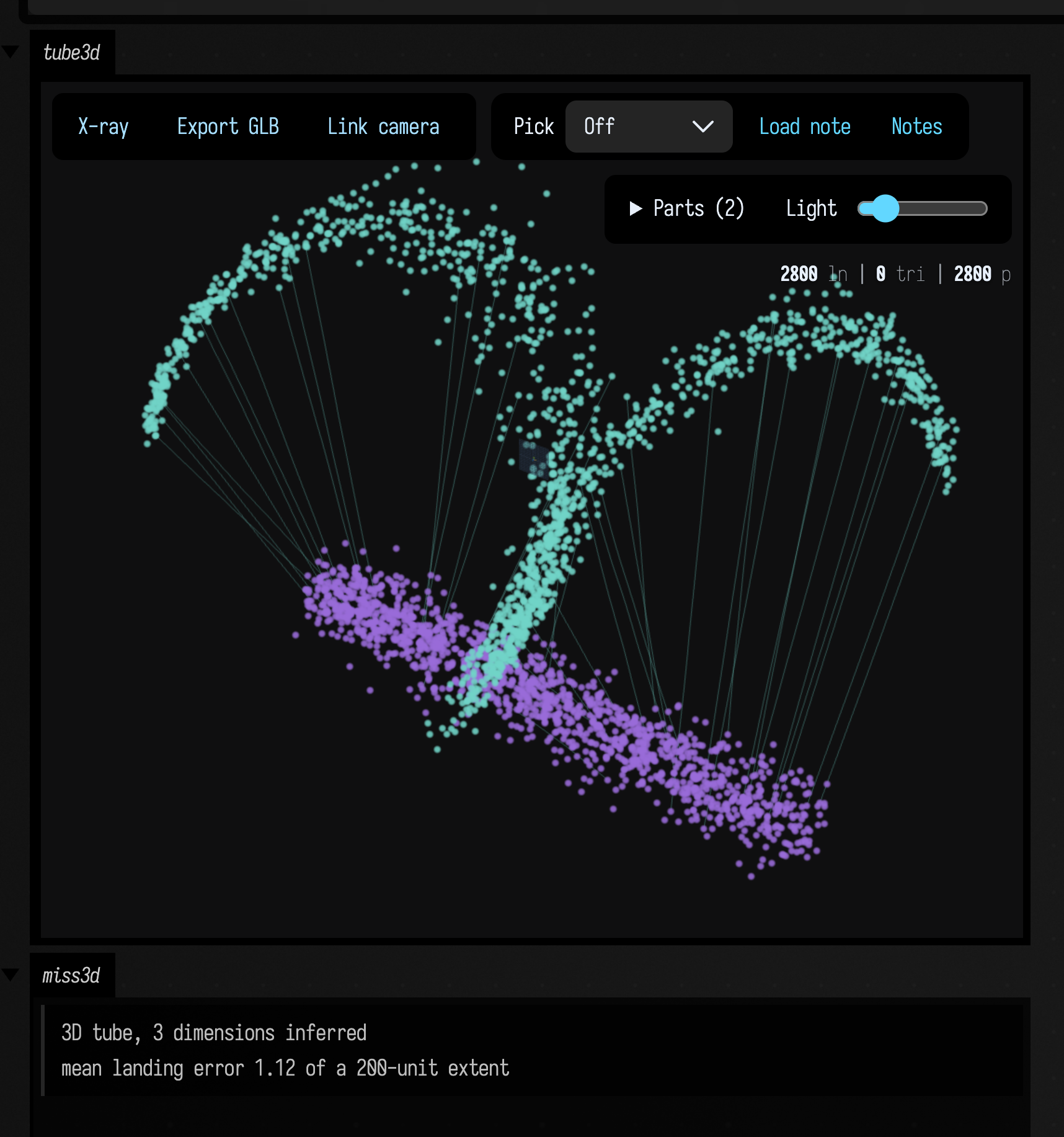

Settings that change the result

A few of FlowMatchOptions's fields account for most of the variation, and the first two have defaults that may surprise you.

activation defaults to leaky rather than tanh. A velocity field has to keep growing away from the data — near t = 0 the right answer is roughly -x, without bound — and a saturating unit cannot, so it bends the far field back on itself. On the ring above, tanh gives about ten times the radial spread of leaky at equal cost, more than any other setting changes it.

finalLearningRate decays the rate linearly across the run, and defaults to doing so. RMSProp rescales the gradient to roughly unit length, so a constant rate keeps taking same-sized steps however close to the answer it already is, and the fit settles at a floor set by the rate. At a constant rate, more steps can leave the result further from its target; with the decay, more steps help. At 6000 steps on the ring, the decay takes the radial spread from 6.3 to 3.0:

fun cloud(points: List<Vec3>, size: Double, c: Vec4, shift: Vec3 = vec(0, 0, 0)): FLine {
    val f = FLine()
    points.forEach { f.moveTo(it + shift) }
    f.pointed = true
    f.pointSize = size
    f.color = c
    return f
}

val target = (0 until 500).map {
    val a = random() * 2 * PI
    vec(100 * cos(a), 100 * sin(a), 0.0)
}

// The ring above, fitted four ways at the same cost; each panel reports its radial spread.
val settings = [
    "leaky, decaying rate (the defaults)" to FlowMatchOptions(steps = 6000, seed = 11),
    "tanh" to FlowMatchOptions(steps = 6000, seed = 11, activation = "tanh"),
    "leaky, constant rate" to FlowMatchOptions(steps = 6000, seed = 11, finalLearningRate = null),
    "tanh, constant rate" to FlowMatchOptions(steps = 6000, seed = 11, activation = "tanh", finalLearningRate = null),
]
:::fold fit four ways, draw them and report the spread
val report = ArrayList<String>()
val panels = settings.flatMapIndexed { i, (label, options) ->
    val samples = flowMatch(target, options = options).sample(300, seed = 12)
    val radii = samples.map { hypot(it.x.toDouble(), it.y.toDouble()) }
    val mean = radii.average()
    val sd = sqrt(radii.sumOf { (it - mean) * (it - mean) } / radii.size)
    report += "${i + 1}. %-38s radius %5.1f +/- %4.1f".format(label, mean, sd)
    val shift = vec(i * 260, 0, 0)
    // The true ring as a thin circle, the samples as dots.
    val ring = FLine()
    for (k in 0..96) {
        val a = k * 2 * PI / 96
        if (k == 0) ring.moveTo(vec(100 * cos(a), 100 * sin(a), 0.0) + shift) else ring.lineTo(vec(100 * cos(a), 100 * sin(a), 0.0) + shift)
    }
    ring.color = vec(0.55, 0.55, 0.62, 0.9)
    val pair: List<FLine> = [ring, cloud(samples, 1.4, vec(0.44, 0.83, 0.78, 1.0), shift)]
    pair
}
lines(panels, w = 1000.0, h = 280.0, fitToSize = true)
markdown("spread", "~~~\n" + report.joinToString("\n") + "\n~~~")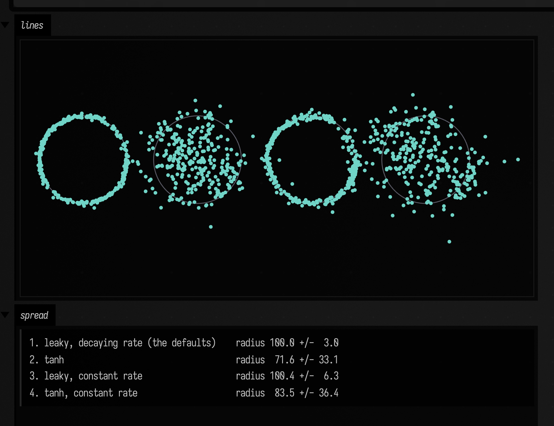

steps is then the quality knob worth reaching for first, and the dominant cost: roughly 0.08 ms per step at the default batch, so 6000 steps is about half a second. hidden defaults to two layers of 64 units, and widening it helps much less than training longer.

FlowMatchField.losses records every step, so a loss still falling at the end means the run was cut short.

Limits of the method

The field is a deformation, so it cannot change topology: no tearing a loop, no joining two strands, no branching. Multiple curves can be carried by one field as long as each has its own source strand of the same kind, and they will approach each other without crossing.

sample returns an unordered cloud. Recovering an FLine from one is a separate problem, which transport sidesteps by moving points you already have and keeping their order.

There is no conditioning input: one field carries one distribution onto one other. And it is a small model — two layers of 64 units suits a few thousand points in two or three dimensions and would not suit an image.

The API is in Machine learning; VectorMLP there is the multi-output regression head that flowMatch trains, which is usable on its own.

FlowMatchField.export() takes a trained field to the GPU as an unrolled GLSL forward pass, and mixtureSource builds the matched-topology source a multi-component target needs. Both are on Particle rules that were trained, along with what the loss on this page does and does not tell you.

See also Stipple transport, which carries a uniform sheet onto a stippled image and animates between images with one network, trained in PyTorch and queried from Field without Python.