Functions to FLine examples (Field graphics)
Plot a function as you build it and you can see what each operation does. Make an envelope for a sound, inspect a transform, or pair two functions and let them draw an ornament.
These examples turn Functions stacks into FLines. We'll start by sampling one stack along x to
make a graph, then use two stacks for the x and y coordinates of a parametric curve.
1D stack: harmonic blend to graph FLine
Start with the ordinary case: one signal, one graph. Once a stack can become a curve, the more elaborate uses are easier to read. This pattern is useful for envelopes, modulation shapes, control signals, and any moment where you need to see a waveform rather than imagine it.
:::static
with(Functions) {
    val x0 = 40.0
    val x1 = 940.0
    val y0 = 50.0
    val y1 = 390.0

    val base = sin(frequency = 2.0, amplitude = 0.72)
    val overtone = sin(frequency = 5.0, phase = 0.35, amplitude = 0.24)
    val detail = valueNoise(seed = 41L, frequency = 22.0, amplitude = 0.07)

    val shaped = ((base + overtone + detail) * hannWindow()).softClip(1.25)

    fun hLine(y: Double, color: Vec4, thickness: Double): FLine = fline {
        moveTo(x0, y)
        lineTo(x1, y)
        this.color = color
        this.thickness = thickness
    }

    fun frame(color: Vec4 = vec(1.0, 1.0, 1.0, 0.28), thickness: Double = 1.6): FLine = fline {
        rect(x0, y0, x1 - x0, y1 - y0)
        this.color = color
        this.thickness = thickness
    }

    val waveform = shaped.toFLine(samples = 900, xScale = 900.0, yScale = 170.0, xOffset = 40.0, yOffset = 220.0).apply {
        color = vec(0.95, 0.92, 0.35, 1.0)
        thickness = 3.2
        stroked = true
        filled = false
    }

    val guides = [
        frame(),
        hLine(220.0, vec(1.0, 1.0, 1.0, 0.35), 1.6),
        hLine(220.0 - 85.0, vec(1.0, 1.0, 1.0, 0.18), 1.0),
        hLine(220.0 + 85.0, vec(1.0, 1.0, 1.0, 0.18), 1.0),
        fline {
            moveTo((x0 + x1) * 0.5, y0)
            lineTo((x0 + x1) * 0.5, y1)
            color = vec(1.0, 1.0, 1.0, 0.12)
            this.thickness = 1.0
        },
    ]

    lines(guides + waveform, channel = "harmonic-graph", w = 980.0, h = 430.0, fitToSize = false)
    markdown("notes", "**1D stack**\n\nsin + overtone + value noise, windowed and soft-clipped.")
}
The ingredients are humble: one base sinusoid, one overtone, a little value noise, then a window and a soft clip to keep the range under control. toFLine(...) does the rest, sampling the stack into drawing space.
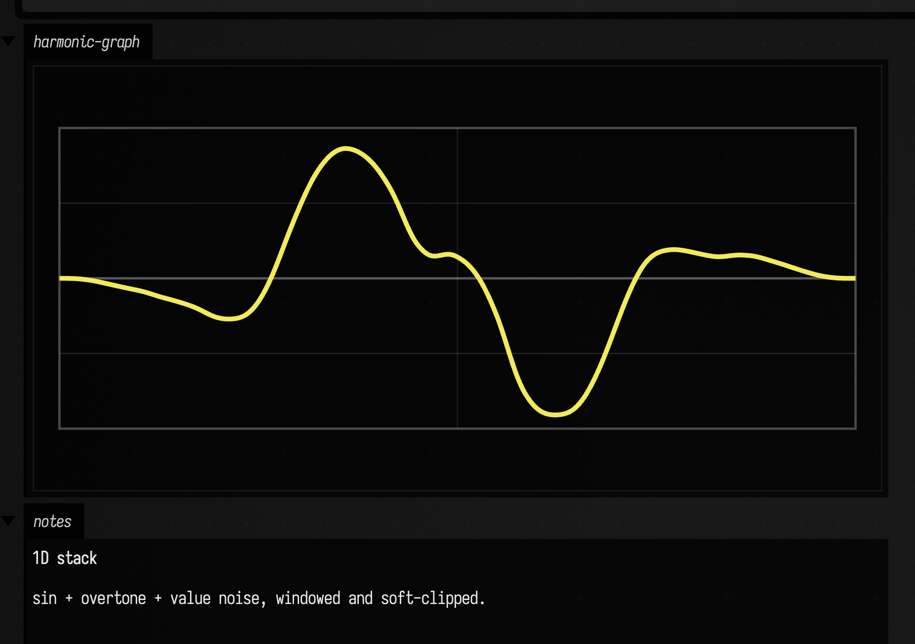
The result still reads as one waveform, but the contribution of each ingredient is visible. This is a useful starting point for envelopes, gesture traces, and "design me a shape" problems. For direct geometry operations after conversion, continue with FLine examples.
1D stack: pulse design, smoothing, and hold
Smooth oscillation is only one side of the system. Edges, gates, bursts, latches, and sample-and-hold behavior matter too. These are the parts that feel like rhythm, switching, or digital control rather than pure tone.
:::static
with(Functions) {
    val x0 = 30.0
    val x1 = 950.0
    val y0 = 40.0
    val y1 = 360.0

    val pulses =
        pulseTrain(period = 0.13, duty = 0.36, rise = 0.01, fall = 0.03, edge = SMOOTH, profile = HANN, amplitude = 1.0)

    val mod = sin(frequency = 1.5, phase = 0.7, amplitude = 0.28)
    val textured = (pulses + mod).clip(1.0)
    val blurred = textured.blur(sigma = 0.015, samples = 48)
    val held = blurred.sampleHold(step = 0.02)

    fun asLine(fn: Functions.Fn, color: Vec4, thickness: Double): FLine = fn.toFLine(samples = 950, xScale = 920.0, yScale = 150.0, xOffset = 30.0, yOffset = 200.0).apply {
        this.color = color
        this.thickness = thickness
    }

    val a = asLine(textured, vec(0.98, 0.63, 0.22, 0.55), 1.3)
    val b = asLine(blurred, vec(0.45, 0.95, 0.72, 0.95), 2.6)
    val c = asLine(held, vec(0.66, 0.82, 1.0, 1.0), 2.0)

    val frame = fline {
        rect(x0, y0, x1 - x0, y1 - y0)
        color = vec(1.0, 1.0, 1.0, 0.22)
        thickness = 1.4
    }

    val center = fline {
        moveTo(x0, 200.0)
        lineTo(x1, 200.0)
        color = vec(1.0, 1.0, 1.0, 0.14)
        thickness = 1.0
    }

    lines(frame, center, a, b, c, channel = "pulse-stack", w = 980.0, h = 400.0, fitToSize = false)
    markdown("notes", "**Pulse stack**\n\npulseTrain → clip → blur → sampleHold")
}
Here the pulse train is the raw material. A slower sine bends it, a blur softens it, and sampleHold(...) turns the result into something more stepped and clocked. Putting the three curves on the same axes makes the transformation easy to compare.
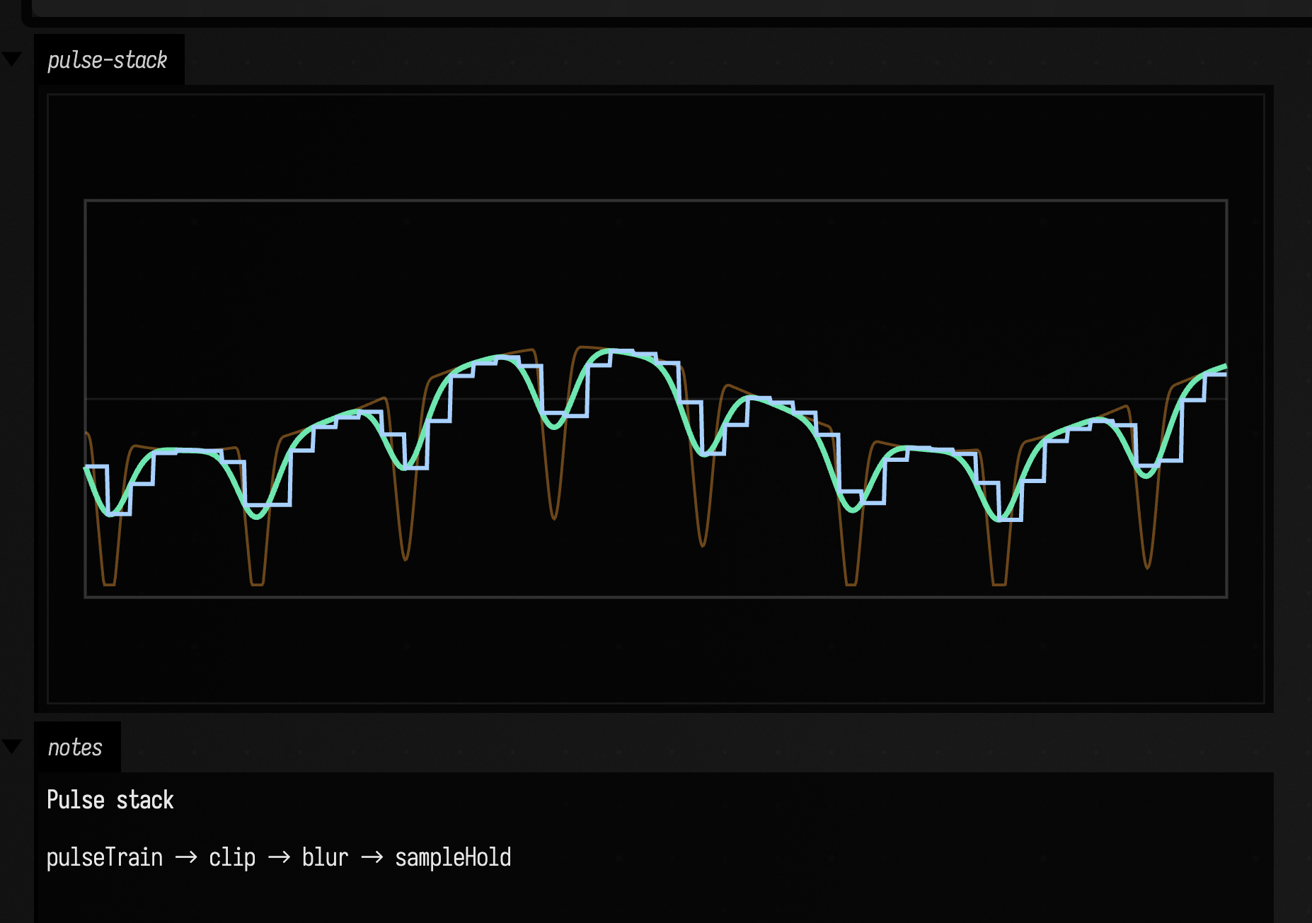
The three traces separate cleanly: one jagged, one softened, one quantized into holds. That side-by-side picture helps when shaping sequencer data, stepped motion, triggers, or control-rate material. For statistical views of similar time-varying data, see the time-domain signal examples.
1D stack: fit a graph to a target (differentiable)
So far we have built stacks by hand. You can also let Field fit one for you. A Functions.Fn is an inspectable graph whose numeric leaves (frequencies, amplitudes, offsets) are tunable "genes". fitBest(target, seed, ...) — the differentiable cousin of the genetic evolve(...) — tunes those numbers by gradient descent (Adam) so the seed's curve slides onto a target signal.
Amplitude and offset are easy to fit. Oscillator frequency is not. The error surface in frequency is bumpy, full of local minima, so a single descent from a wrong frequency gets stuck. fitBest handles that by running several jittered restarts and keeping the best, which gives the search more chances to find the right basin. Here the target is a product of two oscillators and the seed starts with badly wrong frequencies:
:::static
with(Functions) {
    val x0 = 40.0
    val x1 = 940.0
    val y0 = 40.0
    val y1 = 400.0
    val midY = 220.0
    val amp = 150.0

    // A target that is awkward to hand-tune: two oscillators multiplied together.
    val target = cos(2) * sin(1.5, amplitude = 0.8, offset = 0.2)
    // Same *shape*, wrong *numbers* — both frequencies far off, which is the point.
    val seed = cos(3.4) * sin(1.0, amplitude = 2.0)

    /*
    Gradient descent with jittered restarts. A single fitGradient would stall in a
    frequency local-minimum (~0.19); fitBest escapes it. This target is unbounded,
    so fitBest falls back to the finite 0..1 sampling domain.
    */
    val run = fitBest(target, seed, restarts = 16) // RMSE ~0.72 -> ~0.006

    fun asLine(fn: Functions.Fn, color: Vec4, thickness: Double): FLine = fn.toFLine(0.0..1.0, samples = 900, xScale = x1 - x0, yScale = amp, xOffset = x0, yOffset = midY).apply {
        this.color = color
        this.thickness = thickness
    }
    fun hLine(y: Double, color: Vec4, thickness: Double): FLine = fline {
        moveTo(x0, y)
        lineTo(x1, y)
        this.color = color
        this.thickness = thickness
    }
    val frame = fline {
        rect(x0, y0, x1 - x0, y1 - y0)
        color = vec(1.0, 1.0, 1.0, 0.28)
        thickness = 1.6
    }

    val guides = [frame, hLine(midY, vec(1.0, 1.0, 1.0, 0.30), 1.2)]
    val targetLine = asLine(target, vec(0.30, 0.79, 0.94, 1.0), 4.5) // cyan, thick
    val fittedLine = asLine(run.fitted, vec(0.97, 0.45, 0.18, 1.0), 2.2) // orange, thin, on top

    lines(guides + targetLine + fittedLine, channel = "fit-graph", w = 980.0, h = 440.0, fitToSize = false)
    markdown(
        "notes",
        "**fit to target** — target (cyan) vs gradient-fitted (orange), RMSE ${run.finalError.f4}",
    )
    run
}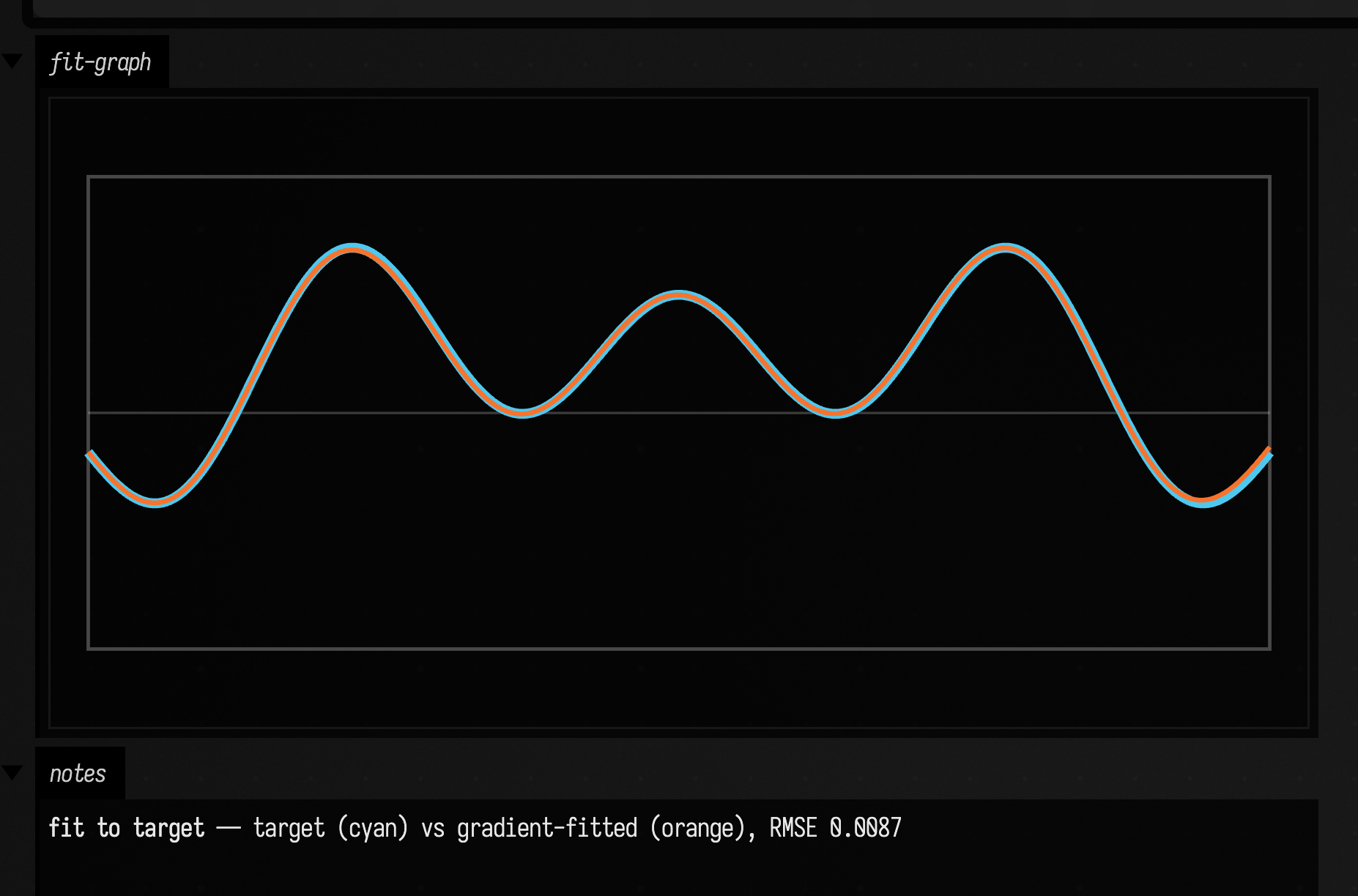
The thin orange (fitted) curve lands right on top of the thick cyan (target): the restarts found the true frequencies, and run reports the RMSE collapsing from ~0.72 to ~0.006. Returning run in the box prints a compact summary with a loss-trajectory sparkline. Reach for fitBest when you have a shape in mind and just need the numbers dialed in; reach for evolve(...) / fitHybrid(...) when the structure itself (which operators) is still unknown.
Watching the descent
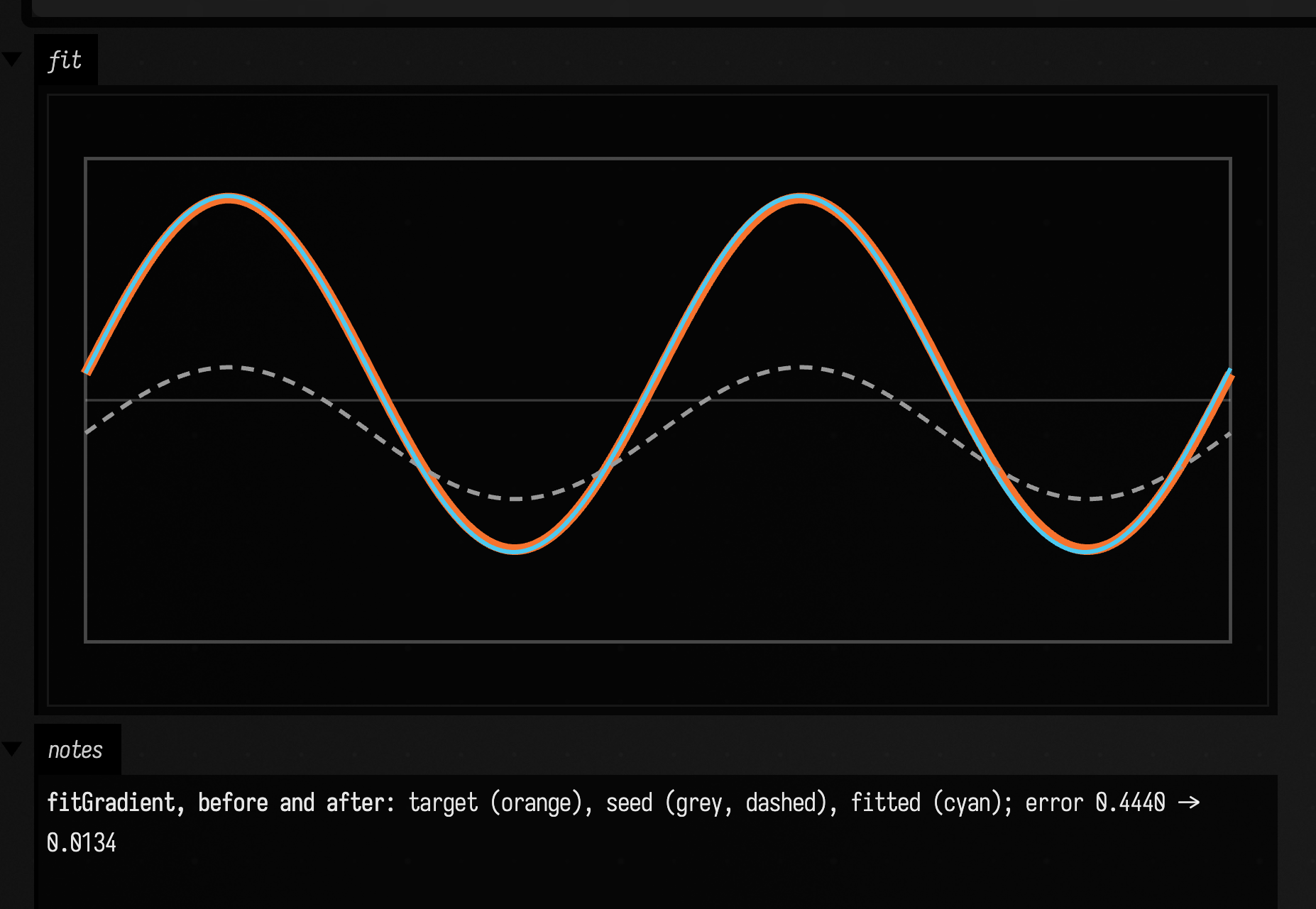
The capture above is the endpoint. The plainer case (a single fitGradient with no restarts, on a
target whose amplitude and offset are wrong but whose frequency is right) shows all three curves at
once: the target, the seed it started from, and where it ended up.
:::static
with(Functions) {
    // The same graph structure as the target, with the wrong numbers in it: a fifth of the
    // amplitude and the offset the wrong way. One fitGradient, no restarts.
    val target = sin(frequency = 2.0, amplitude = 0.8, offset = 0.12)
    val seed = sin(frequency = 2.0, amplitude = 0.30, offset = -0.15)
    val run = fitGradient(target = target, seed = seed, iterations = 400, lr = 0.05, samples = 160, rngSeed = 0L)

    :::fold the plot frame: 900 x 380 px, y up, values -1.1..1.1
    val x0 = 40.0
    val x1 = 940.0
    val y0 = 30.0
    val y1 = 410.0
    val lo = -1.1
    val hi = 1.1
    val yScale = -(y1 - y0) / (hi - lo)
    val zeroY = y1 + lo * (y1 - y0) / (hi - lo)
    fun curve(fn: Functions.Fn, color: Vec4, thickness: Double, dashed: Boolean = false): List<FLine> {
        val line = fn.toFLine(0.0..1.0, samples = 600, xScale = x1 - x0, yScale = yScale, xOffset = x0, yOffset = zeroY)
        val parts = if (dashed) line.byDashing(10f, 7f) else [line]
        return parts.onEach {
            it.color = color
            it.thickness = thickness
        }
    }
    val guides = [
        fline {
            rect(x0, y0, x1 - x0, y1 - y0)
            color = vec(1.0, 1.0, 1.0, 0.28)
            thickness = 1.6
        },
        fline {
            moveTo(x0, zeroY)
            lineTo(x1, zeroY)
            color = vec(1.0, 1.0, 1.0, 0.30)
            thickness = 1.2
        },
    ]
    val orange = vec(0.97, 0.45, 0.18, 1.0)
    val cyan = vec(0.30, 0.79, 0.94, 1.0)
    val grey = vec(0.6, 0.6, 0.6, 1.0)
    val violet = vec(0.66, 0.50, 0.98, 1.0)
    val green = vec(0.45, 0.85, 0.45, 1.0)
    val pink = vec(0.96, 0.45, 0.72, 1.0)
    :::endfold

    lines(
        guides + curve(target, orange, 5.0) + curve(seed, grey, 2.0, dashed = true) + curve(run.fitted, cyan, 2.0),
        channel = "fit",
        w = 980.0,
        h = 440.0,
        fitToSize = false,
    )
    markdown(
        "notes",
        "**fitGradient, before and after**: target (orange), seed (grey, dashed), fitted (cyan); " +
            "error ${run.initialError.f4} -> ${run.finalError.f4}",
    )
}
And the descent itself, from iteration 0 to 320, with the early iterations shown longest because that is where the curve moves. Each frame is its own
fitGradient run, truncated at that iteration count, so the error printed under it belongs to that run:
:::static
/*
Iteration counts bunched where the curve moves, each held for three frames, then the last held.
Each is its own fitGradient run, truncated at that count, so the error belongs to that run.
*/
val steps = [0, 1, 2, 3, 4, 5, 6, 8, 10, 12, 14, 16, 18, 20, 22, 24, 27, 30, 34, 38, 42, 48, 56, 64, 80, 96, 128, 160, 224, 320]
var frameIndex = 0
loop {
    val k = steps[minOf(frameIndex / 3, steps.size - 1)]
    frameIndex++
    with(Functions) {
        val target = sin(frequency = 2.0, amplitude = 0.8, offset = 0.12)
        val seed = sin(frequency = 2.0, amplitude = 0.30, offset = -0.15)
        val run =
            fitGradient(target = target, seed = seed, iterations = k, lr = 0.05, samples = 160, rngSeed = 0L)
        :::fold the plot frame: 900 x 380 px, y up, values -1.1..1.1
        val x0 = 40.0
        val x1 = 940.0
        val y0 = 30.0
        val y1 = 410.0
        val lo = -1.1
        val hi = 1.1
        val yScale = -(y1 - y0) / (hi - lo)
        val zeroY = y1 + lo * (y1 - y0) / (hi - lo)
        fun curve(fn: Functions.Fn, color: Vec4, thickness: Double, dashed: Boolean = false): List<FLine> {
            val line =
                fn.toFLine(0.0..1.0, samples = 600, xScale = x1 - x0, yScale = yScale, xOffset = x0, yOffset = zeroY)
            val parts = if (dashed) line.byDashing(10f, 7f) else [line]
            return parts.onEach {
                it.color = color
                it.thickness = thickness
            }
        }
        val guides = [
            fline {
                rect(x0, y0, x1 - x0, y1 - y0)
                color = vec(1.0, 1.0, 1.0, 0.28)
                thickness = 1.6
            },
            fline {
                moveTo(x0, zeroY)
                lineTo(x1, zeroY)
                color = vec(1.0, 1.0, 1.0, 0.30)
                thickness = 1.2
            },
        ]
        val orange = vec(0.97, 0.45, 0.18, 1.0)
        val cyan = vec(0.30, 0.79, 0.94, 1.0)
        val grey = vec(0.6, 0.6, 0.6, 1.0)
        val violet = vec(0.66, 0.50, 0.98, 1.0)
        val green = vec(0.45, 0.85, 0.45, 1.0)
        val pink = vec(0.96, 0.45, 0.72, 1.0)
        :::endfold

        lines(
            guides + curve(target, orange, 5.0) + curve(run.fitted, cyan, 2.0),
            channel = "descent",
            w = 980.0,
            h = 440.0,
            fitToSize = false,
        )
        markdown("iteration", "**iteration $k**: error ${run.finalError.f4}")
    }
    frame()
}
Watch which parameter moves first; the error number alone hides it. Amplitude is essentially found by iteration 8 (the peaks already match) and the error is still 0.1030, because what is left is the vertical offset (the troughs sit shallow) and a small phase lead. Those take the remaining three hundred iterations to close: 0.0248 by iteration 48, 0.0044 at 320. A single error figure would have read as "nearly converged" three hundred iterations early.
2D stack: separate x(t) and y(t) Functions
A function stack does not have to mean "height over x". Two of them can steer a path instead: one controls horizontal position, the other vertical.
:::static
with(Functions) {
    val tDomain = 0.0..1.0
    val cx = 500.0
    val cy = 250.0

    val xFn =
        (sin(frequency = 3.0, phase = 0.2, amplitude = 1.0, domain = tDomain) +
                sin(frequency = 9.0, phase = 1.1, amplitude = 0.18, domain = tDomain))
            .softClip(1.15)

    val yFn =
        (sin(frequency = 4.0, phase = 1.2, amplitude = 1.0, domain = tDomain) +
                valueNoise(seed = 88L, frequency = 16.0, amplitude = 0.1, domain = tDomain))
            .softClip(1.2)

    fun parametric(xf: Functions.Fn, yf: Functions.Fn, samples: Int = 1400): FLine {
        val f = FLine()
        f.breakNext()
        for (i in 0 until samples) {
            val t = tDomain.lerp(i.toDouble() / (samples - 1).coerceAtLeast(1).toDouble())
            val x = cx + xf.eval(t) * 290.0
            val y = cy + yf.eval(t) * 190.0
            f.lineTo(x, y)
        }
        return f
    }

    val frame = fline {
        rect(120.0, 60.0, 760.0, 380.0)
        color = vec(1.0, 1.0, 1.0, 0.24)
        thickness = 1.4
    }

    val cross = [
        fline {
            moveTo(120.0, cy)
            lineTo(880.0, cy)
            color = vec(1.0, 1.0, 1.0, 0.12)
            thickness = 1.0
        },
        fline {
            moveTo(cx, 60.0)
            lineTo(cx, 440.0)
            color = vec(1.0, 1.0, 1.0, 0.12)
            thickness = 1.0
        },
    ]

    val curve = parametric(xFn, yFn).apply {
        color = vec(0.98, 0.9, 0.32, 0.95)
        thickness = 2.3
    }

    lines([frame] + cross + curve, channel = "xy-parametric", w = 1000.0, h = 500.0, fitToSize = false)
    markdown("notes", "**2D parametric**\n\nx(t) and y(t) are independent Functions stacks.")
}
xFn and yFn stay independent until the moment of sampling, where parametric(...) evaluates them together. The shape of the path comes from how the two relate.
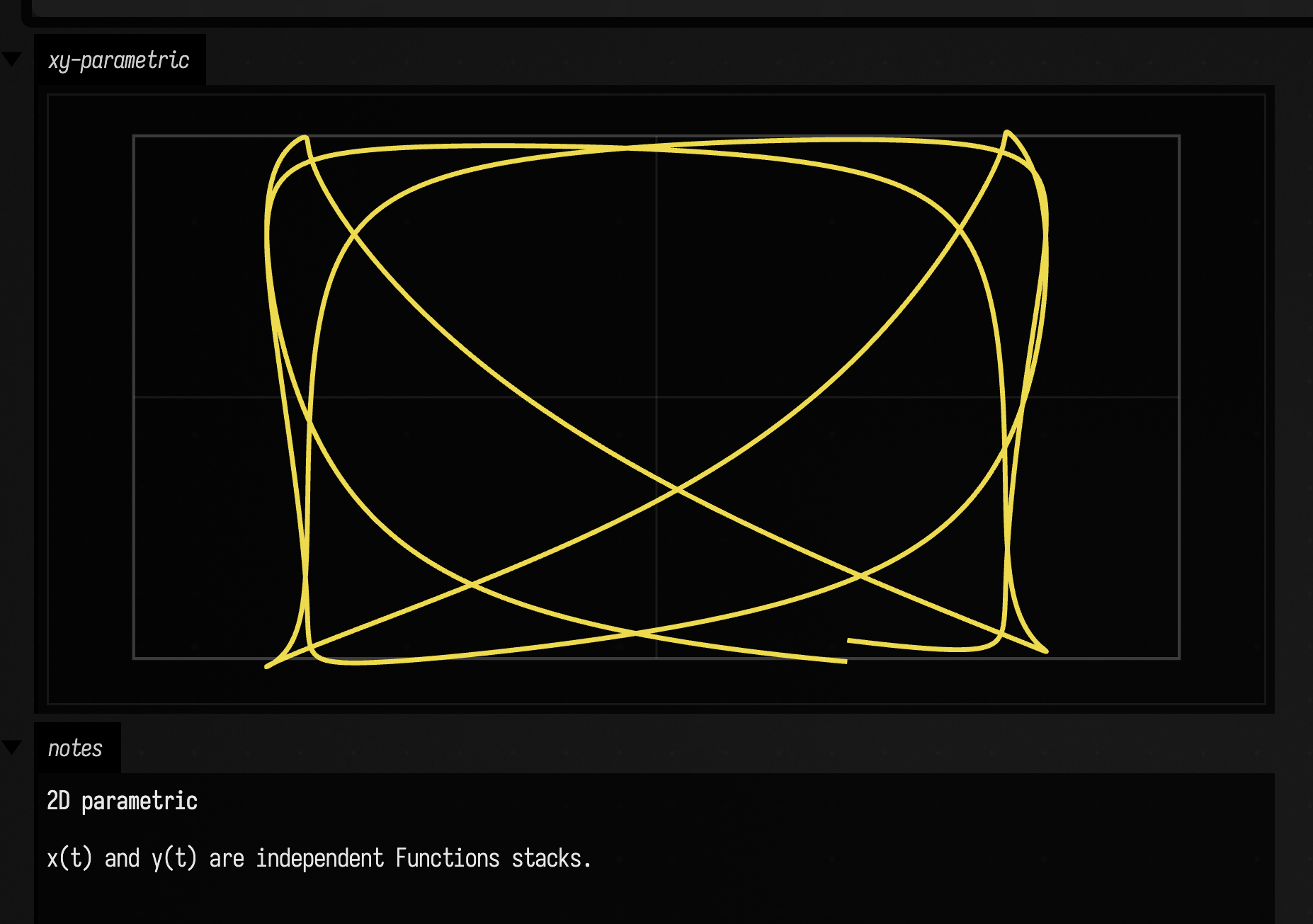
The curve has different tempos on its two axes, so it reads as an orbit, a trajectory, or ornament rather than a graph. This is a workhorse pattern for parametric drawing. For lower-level path editing once you have the curve, see FLine examples.
2D stack: noisy rosette with windowed arc energy
Sometimes the useful coordinates are radius and angle, not x and y. That shift suits rosettes, emblems, radial plots, circular choreography, and drawings that grow outward rather than march left to right.
:::static
with(Functions) {
    val tDomain = 0.0..1.0
    val cx = 500.0
    val cy = 250.0

    val radial =
        (one(tDomain) * 0.62 +
                pulseTrain(period = 0.25, duty = 0.5, profile = TRIANGLE, amplitude = 0.22, domain = tDomain) +
                valueNoise(seed = 5L, frequency = 14.0, amplitude = 0.05, domain = tDomain))
            .clamp(0.12, 1.0)

    val theta = ramp(start = 0.0, end = 1.0, domain = tDomain) * Math.PI * 2.0 * 6.0

    // Explicit x/y from radial + theta, sampled directly for clarity.
    val line = FLine()
    line.breakNext()
    val samples = 1800
    for (i in 0 until samples) {
        val t = tDomain.lerp(i.toDouble() / (samples - 1).coerceAtLeast(1).toDouble())
        val r = radial.eval(t)
        val ang = theta.eval(t)
        val x = cx + kotlin.math.cos(ang) * r * 280.0
        val y = cy + kotlin.math.sin(ang) * r * 210.0
        line.lineTo(x, y)
    }

    line.color = vec(0.62, 0.95, 1.0, 0.95)
    line.thickness = 2.0

    val frame = fline {
        rect(120.0, 60.0, 760.0, 380.0)
        color = vec(1.0, 1.0, 1.0, 0.22)
        thickness = 1.4
    }

    val ringGuide = fline {
        circle(cx, cy, 210.0, segments = 220)
        color = vec(1.0, 1.0, 1.0, 0.1)
        thickness = 1.0
    }

    lines(frame, ringGuide, line, channel = "xy-rosette", w = 1000.0, h = 500.0, fitToSize = false)
    markdown("notes", "**2D rosette**\n\nradial(t) + angle(t) stack mapped into x/y.")
}
The code builds the motion in polar terms first: radius from pulseTrain(...) and valueNoise(...), angle from a ramp. Only after that does it convert to cartesian coordinates. The explicit sampling loop keeps the conversion visible.
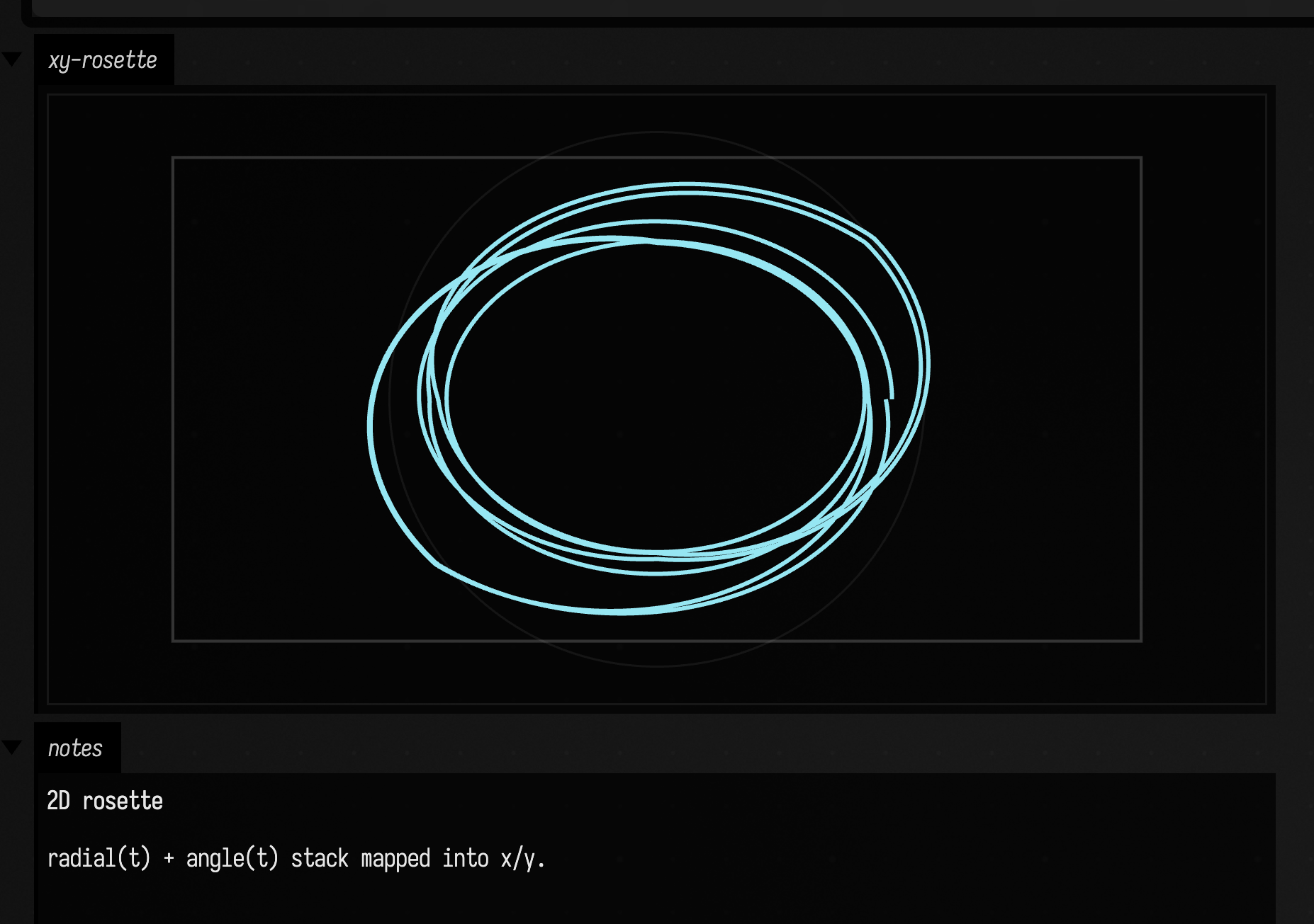
The radius creates petals and breaths; the angle decides how they are laid around the circle. This is a strong pattern for radial ornaments, animated emblems, and circular plotting systems. For color strategies that pair well with this kind of geometry, see Colors examples.
Diff runner: edit a stack and capture the new look
With Functions, a small edit can materially change the drawing. That makes diff examples useful: you can see what a new ingredient actually changed.
:::before
with(Functions) {
    val a = sin(frequency = 2.0, amplitude = 0.7)
    val b = pulseTrain(period = 0.2, duty = 0.35, amplitude = 0.35)
    val f = (a + b).softClip(1.0)

    val line = f.toFLine(samples = 900, xScale = 900.0, yScale = 160.0, xOffset = 40.0, yOffset = 220.0).apply {
        color = vec(1.0, 0.75, 0.4, 1.0)
        thickness = 2.0
    }

    val frame = fline {
        rect(40.0, 50.0, 900.0, 340.0)
        color = vec(1.0, 1.0, 1.0, 0.22)
        thickness = 1.3
    }

    lines(frame, line, channel = "edited-stack", w = 980.0, h = 420.0, fitToSize = false)
    markdown("notes", "**Before**: simple sin + pulse stack.")
}
:::after
with(Functions) {
    val a = sin(frequency = 2.0, amplitude = 0.7)
    val b = pulseTrain(period = 0.2, duty = 0.35, rise = 0.01, fall = 0.025, profile = HANN, amplitude = 0.35)
    val detail = fbm(seed = 77L, frequency = 4.0, amplitude = 0.12, octaves = 4)
    val f = (a + b + detail).softClip(1.22)

    val line = f.toFLine(samples = 900, xScale = 900.0, yScale = 160.0, xOffset = 40.0, yOffset = 220.0).apply {
        color = vec(0.58, 0.93, 1.0, 1.0)
        thickness = 2.6
    }

    val frame = fline {
        rect(40.0, 50.0, 900.0, 340.0)
        color = vec(1.0, 1.0, 1.0, 0.24)
        thickness = 1.4
    }

    val center = fline {
        moveTo(40.0, 220.0)
        lineTo(940.0, 220.0)
        color = vec(1.0, 1.0, 1.0, 0.12)
        thickness = 1.0
    }

    lines(frame, center, line, channel = "edited-stack", w = 980.0, h = 420.0, fitToSize = false)
    markdown("notes", "**After**: shaped pulse + fbm detail + stronger soft clip.")
}
The diff keeps the frame and scale fixed and changes only the stack: a more shaped pulse, a little fbm(...) detail, and a firmer soft clip. The picture stays recognisably the same drawing.
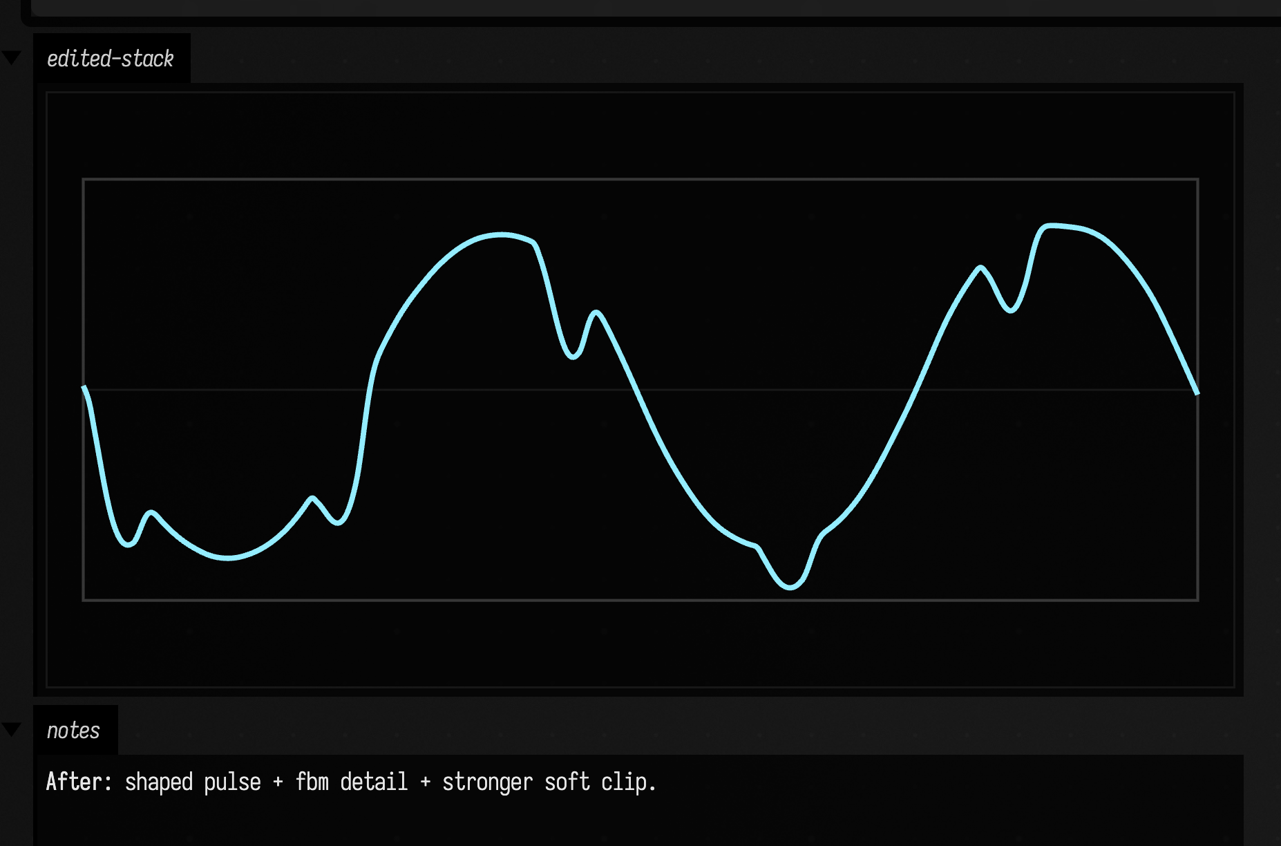
The broad contour survives, while the surface gains character. The expanded reference below is the place to browse the API once the main patterns are familiar.
Domains and timeline composition
Fn has one public interval: domain. Arithmetic intersects domains, replacement and piecewise tools expand domains when they truly need to, and timeline chunks keep their source interval separate from the interval where they are placed. Domains works through that model on its own; this section is about the composition helpers built over it.
Unless a constructor says otherwise, a fresh Fn starts with Domain.DEFAULT, which is 0.0..1.0. Oscillators are the exception: the periodic constructors (sin, cos, saw, triangle, square) and the pulseTrain/impulseTrain/pulseBurst family default to Domain.ALL, because a periodic signal is genuinely defined on all of R. Use domain = ... to change the construction interval, use over (...) to relabel or place an existing function, and use / all when any other unbounded function is genuinely meant. Enumerating an unbounded function (toDoubleArray, sampleUniform, plot, stream, and the rest of the sampling surface) with no explicit interval is safe: it previews over a finite window (0.0..1.0) rather than trying to walk the whole real line.
The declarative timeline layer is thin Kotlin over those same pieces. over sets the resulting function domain, stretch remaps the left-hand domain into a new one, then concatenates two functions, overlapping creates an overlapped pair, and / pipes a function through reusable transforms. through and pipe are the readable aliases; / is the compact style that matches the audio section. The transform all is the terse form of "set the domain to Domain.ALL", so sin(0.5) / all is the compact unbounded signal spelling. Because over and stretch are infix calls, keep the target range in parentheses; for longer arithmetic stacks, wrap the left side too.
Numeric parameters on these helpers accept Kotlin Numbers and can also be Fns. Literals like overlap = 1, overlap = 0.1, or slower(2) are just the constant-function case; an Fn parameter is sampled near where it applies, such as the midpoint of a join's overlap, or the current slot/grain for random-repeat style transforms. The terse 0.25 form is a parameter signal, so it does not narrow the domain of the function it configures.
domain = ... vs over ...
For a periodic function like pulseTrain, these two forms usually produce the same sampled values:
val a = pulseTrain(period = 0.08, duty = 0.35, domain = 0.0..0.8)
val b = pulseTrain(period = 0.08, duty = 0.35) over (0.0..0.8)
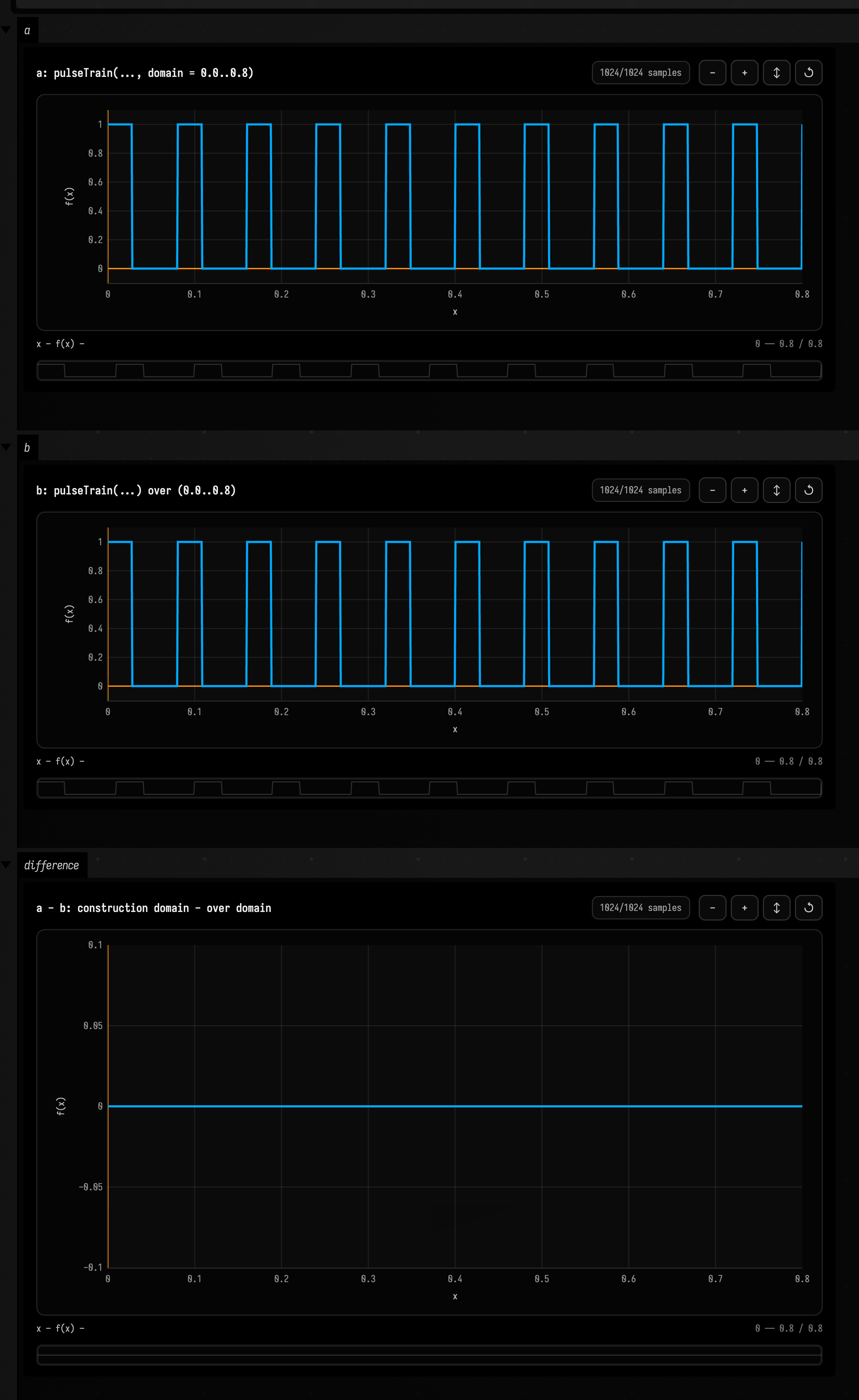
The first form builds the pulse train with 0.0..0.8 as its construction-time domain. The second form builds the pulse train with its default unbounded domain (Domain.ALL), then replaces the public Fn.domain with 0.0..0.8. Because pulseTrain computes phase from x, period, duty, and phase rather than from domain-normalized position, the two functions are effectively equivalent here. The box below plots a, then b, then a - b: the same ten pulses twice, and a flat zero line.
:::static
with(Functions) {
    val a = pulseTrain(period = 0.08, duty = 0.35, domain = 0.0..0.8)
    val b = pulseTrain(period = 0.08, duty = 0.35) over (0.0..0.8)

    a.plot(
        "a",
        domain(0.0..0.8),
        heightPx = 200,
        title = "a: pulseTrain(..., domain = 0.0..0.8)",
        yDomain = domain((-0.1)..1.1),
    )
    b.plot(
        "b",
        domain(0.0..0.8),
        heightPx = 200,
        title = "b: pulseTrain(...) over (0.0..0.8)",
        yDomain = domain((-0.1)..1.1),
    )

    (a - b).plot(
        "difference",
        domain(0.0..0.8),
        title = "a - b: construction domain - over domain",
        yDomain = domain((-0.1)..0.1),
    )
}
The difference matters for functions where the domain is part of the math. Windows and ramps care about their construction domain because they normalize x across that interval:
val shaped = hannWindow(0.0..0.8)
val relabeled = hannWindow() over (0.0..0.8)
hannWindow(0.0..0.8) means "shape the whole Hann curve across 0.0..0.8". hannWindow() over (0.0..0.8) means "make a Hann curve over its default 0.0..1.0 construction domain, then relabel its valid interval".
:::static
with(Functions) {
    val shaped = hannWindow(0.0..0.8)
    val relabeled = hannWindow() over (0.0..0.8)

    (shaped - relabeled).plot(
        "plot",
        domain(0.0..0.8),
        title = "hannWindow: construction domain - over domain",
        yDomain = domain((-1.0)..1.0),
    )
}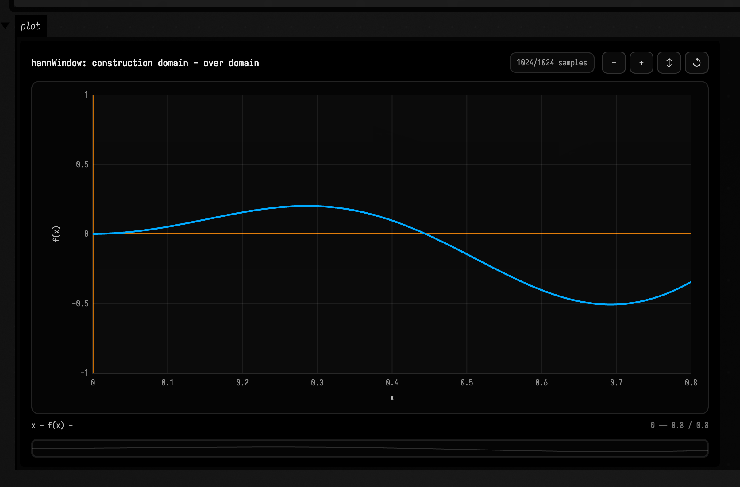
The short rule is: use domain = ... when the construction interval should affect internals, and use over ... when you want post-hoc timeline placement, trimming, or extent declaration. For pure periodic signals those often coincide. For domain-normalized shapes, they do not.
over ... vs stretch ...
over changes only the public domain. stretch changes the x-coordinate lookup, so the whole source domain is replayed across the target domain:
val relabeled = sin(5.0) over (0.0..10.0)
val stretched = sin(5.0) stretch (0.0..10.0)
val alsoStretched = sin(5.0) / stretch(0.0..10.0)
Stretching needs finite source and target domains. If the source is unbounded, give it a finite source interval first:
val fromSlice = (sin(0.5) / all).stretchFrom(from = 0.0..1.0, to = 0.0..12.0)The default stretch is linear in normalized time. stretchSmooth(...), stretchSmoother(...), and stretchBy(..., warp = someFn) warp that normalized time before sampling the source:
val linear = pulseTrain(0.1) stretch (0.0..4.0)
val eased = pulseTrain(0.1).stretchSmooth(0.0..4.0)
val softer = pulseTrain(0.1) / stretchSmoother(0.0..4.0)
val custom = pulseTrain(0.1).stretchBy(0.0..4.0, warp = smoothStep(0.0, 1.0))
with(Functions) {
val tone = ((sin(5) * 1.4) / delay(0.4) / slower(2)) over (0.0..10.0)
val forever = sin(0.25) / all
val stretchedTone = sin(5.0) stretch (0.0..10.0)
val easedTone = sin(5.0) / stretchSmoother(0.0..10.0)
val a = sin(2.0) over (0.0..1.0)
val b = pulseTrain(period = 0.12, duty = 0.35, domain = 0.0..1.0)
val phrase = a then ((b / softClipBy(1.5)) over (0.0..1.0))
val pad = (a overlapping 0.5) with (sin(7.0) / gain(0.35))
val alsoPad = a.overlapping(0.5, sin(7.0) / gain(0.35))
val palette = [
sin(2.0) over (0.0..1.0),
saw(0.12) over (0.0..0.6),
pulseTrain(period = 0.08, duty = 0.35, domain = 0.0..0.8),
]
val movingOverlap = ramp(0.02, 0.18, 0.0..10.0)
val melody = palette.sequence(overlap = movingOverlap)
val endless =
(palette.randomSequence(seed = 4, overlap = 0.05, slot = ramp(0.18, 0.42, 0.0..10.0)) / all) over (0.0..10.0)
val shuffled = palette.shuffleLoop(seed = 9, overlap = 0.12) over (0.0..12.0)
val morph = palette.morph(ramp(0.0, 2.0, 0.0..1.0))
val tornTape =
(sin(5.0) /
slower(ramp(0.8, 1.6, 0.0..4.0)) /
turbulence(amount = 0.035, frequency = 11.0) /
randomCopyPaste(grain = ramp(0.08, 0.2, 0.0..4.0), seed = 5)) over (0.0..4.0)
}Shaping signals: the Functions transform pipeline
The reference below lists every constructor and combiner in isolation. This section is the
opposite view: how the small handful of infix operators fit together into a pipeline, so
a stack like pulseBurst(10) through gain(0.6) over (0.0..4.0) reads on sight and you can
write your own without hunting through the catalogue.
The mental model
A pipeline has two kinds of thing in it:
- a source
Fn— a signal you can sample at anyx(ramp,cos,pulseBurst, …); - a
FnTransform— a reusable edit, a packaged(Fn) -> Fn, produced by a builder likegain(0.6),delay(0.1),lowPass(0.08), orsoftClipBy(1.2).
You shape a source by sending it through a transform. The result is another Fn, so you
can send that through the next transform, and so on. A FnTransform holds no state and can be reused across as many sources as you like, so
build a shaping chain once, name it, and apply it everywhere.
The operators
| Operator | Shape | Meaning |
|---|---|---|
source through t |
Fn through FnTransform → Fn |
Apply transform t to the source. |
source pipe t |
Fn pipe FnTransform → Fn |
Readable alias for through. |
source / t |
Fn / FnTransform → Fn |
Compact alias for through (matches the audio style). |
t1 then t2 |
FnTransform then FnTransform → FnTransform |
Compose two transforms into one (apply t1, then t2). |
t1 / t2 |
FnTransform / FnTransform → FnTransform |
Compact alias for composing transforms. |
source over (a..b) |
Fn over ClosedRange → Fn |
Relabel the public domain to a..b (placement, no resampling). |
source stretch (a..b) |
Fn stretch ClosedRange → Fn |
Remap the source's domain across a..b (replays the whole source over the new interval). |
a then b |
Fn then Fn → Fn |
Concatenate two functions end-to-end on a timeline. |
a overlapping n with b |
Fn overlapping Number with Fn → Fn |
Join a and b with an n-wide crossfade. |
Two overloads share a name. then composes transforms when both sides are FnTransform
(gain(0.6) then lowPass(0.08)), and concatenates functions when both sides are Fn
(intro then verse). The compiler picks by operand type; the editor's completion leans on the
same distinction (below). For the over / stretch distinction (relabelling versus
remapping), see over ... vs stretch ... above; here we only use them to
place a finished pipeline on a timeline.
What the shapers actually do
A waveshaper reads most easily from its transfer curve: push a rising ramp through it, and the
plotted result is the shape it imposes on whatever you send it. Four of them, over an input sweep
of -1.5..1.5, against the ramp itself as a dashed reference:
val sweep = ramp(-1.5, 1.5) over Functions.Domain.of(0.0, 1.0)

sweep.fold(0.7) // reflects back at the threshold
sweep.softClip(2.5) // a bounded S, smooth everywhere
sweep.chebyshev(3) // the 3rd Chebyshev polynomial
sweep.rectify(Functions.RectifyMode.FULL) // absolute value, folded about zero
:::static
with(Functions) {
// Push a rising ramp through each shaper: what comes out is the shape it imposes.
val sweep = ramp(-1.5, 1.5) over Functions.Domain.of(0.0, 1.0)
:::fold the plot frame: 900 x 380 px, y up, values -1.7..1.7
val x0 = 40.0
val x1 = 940.0
val y0 = 30.0
val y1 = 410.0
val lo = -1.7
val hi = 1.7
val yScale = -(y1 - y0) / (hi - lo)
val zeroY = y1 + lo * (y1 - y0) / (hi - lo)
fun curve(fn: Functions.Fn, color: Vec4, thickness: Double, dashed: Boolean = false): List<FLine> {
val line = fn.toFLine(0.0..1.0, samples = 600, xScale = x1 - x0, yScale = yScale, xOffset = x0, yOffset = zeroY)
val parts = if (dashed) line.byDashing(10f, 7f) else [line]
return parts.onEach {
it.color = color
it.thickness = thickness
}
}
val guides = [
fline {
rect(x0, y0, x1 - x0, y1 - y0)
color = vec(1.0, 1.0, 1.0, 0.28)
thickness = 1.6
},
fline {
moveTo(x0, zeroY)
lineTo(x1, zeroY)
color = vec(1.0, 1.0, 1.0, 0.30)
thickness = 1.2
},
]
val orange = vec(0.97, 0.45, 0.18, 1.0)
val cyan = vec(0.30, 0.79, 0.94, 1.0)
val grey = vec(0.6, 0.6, 0.6, 1.0)
val violet = vec(0.66, 0.50, 0.98, 1.0)
val green = vec(0.45, 0.85, 0.45, 1.0)
val pink = vec(0.96, 0.45, 0.72, 1.0)
:::endfold
lines(
guides +
curve(sweep, grey, 2.0, dashed = true) +
curve(sweep.fold(0.7), cyan, 2.4) +
curve(sweep.softClip(2.5), orange, 2.4) +
curve(sweep.chebyshev(3), violet, 2.4) +
curve(sweep.rectify(Functions.RectifyMode.FULL), green, 2.4),
channel = "transfer",
w = 980.0,
h = 440.0,
fitToSize = false,
)
markdown(
"notes",
"**transfer curves over a -1.5..1.5 sweep**: input ramp (grey, dashed), fold(0.7) (cyan), " +
"softClip(2.5) (orange), chebyshev(3) (violet), rectify(FULL) (green)",
)
}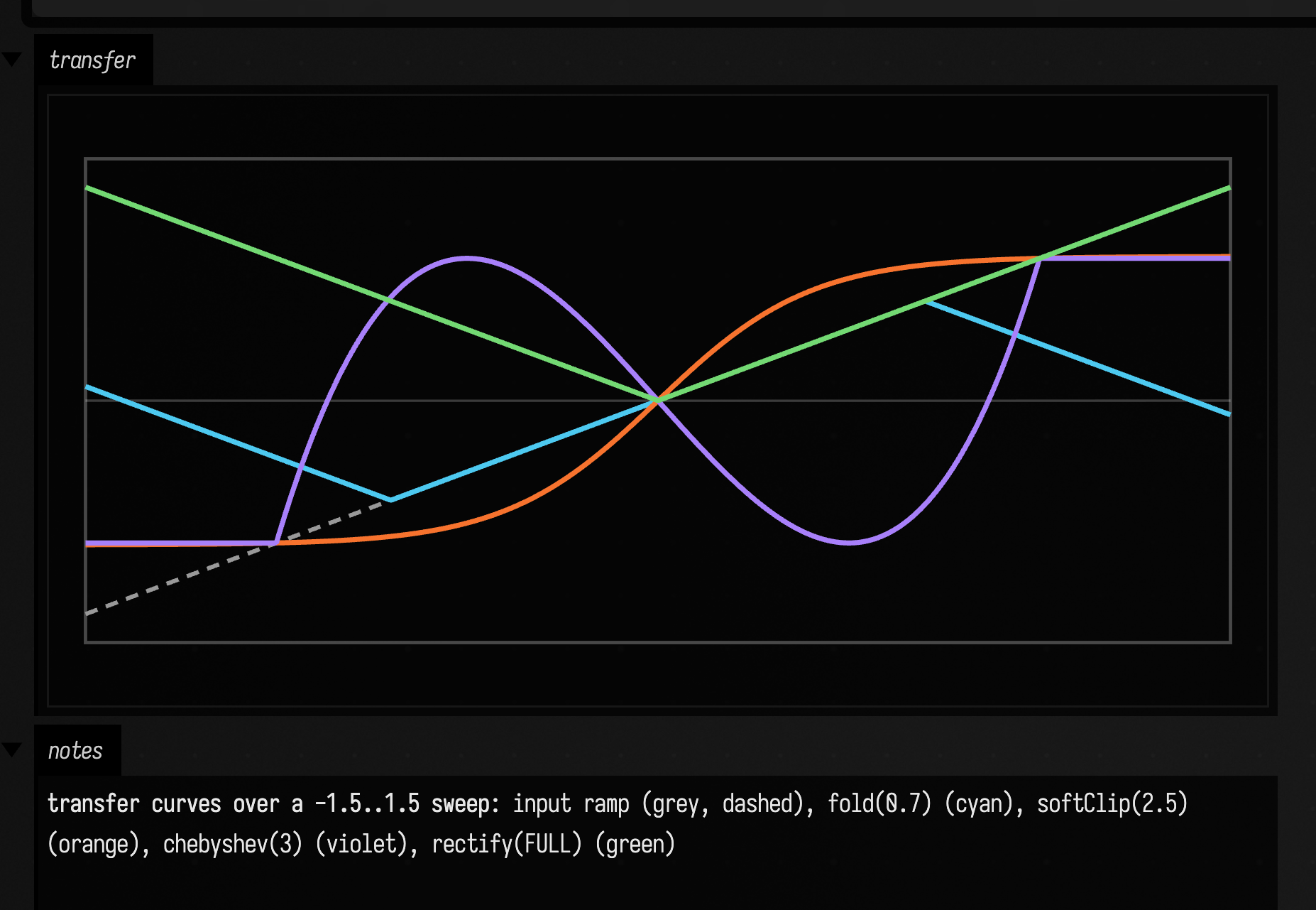
fold reflects rather than flattens, so it keeps adding harmonics where a clipper stops; softClip
is bounded and smooth everywhere, so it has no corner to alias off; chebyshev(3) is a polynomial,
so it maps a unit cosine to a pure third harmonic rather than a smear.
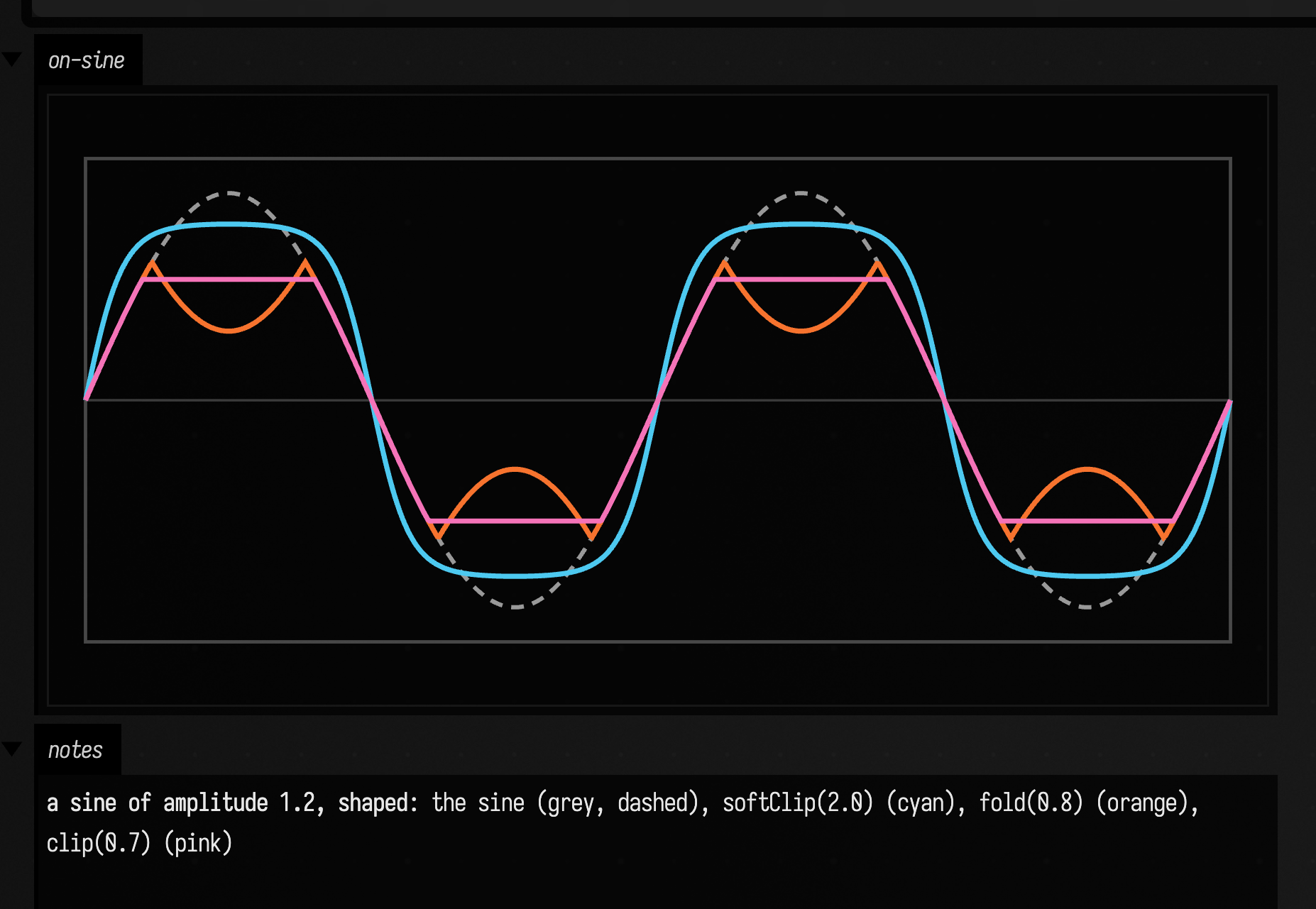
Now on real signal rather than on a ramp: a 1.2-amplitude sine, so each shaper has something to
bite on. clip appears here and not above, because it is the only member of the family with
corners in it:
:::static
with(Functions) {
    val tone = sin(frequency = 2.0, amplitude = 1.2)

    :::fold the plot frame: 900 x 380 px, y up, values -1.4..1.4
    val x0 = 40.0
    val x1 = 940.0
    val y0 = 30.0
    val y1 = 410.0
    val lo = -1.4
    val hi = 1.4
    val yScale = -(y1 - y0) / (hi - lo)
    val zeroY = y1 + lo * (y1 - y0) / (hi - lo)
    fun curve(fn: Functions.Fn, color: Vec4, thickness: Double, dashed: Boolean = false): List<FLine> {
        val line = fn.toFLine(0.0..1.0, samples = 600, xScale = x1 - x0, yScale = yScale, xOffset = x0, yOffset = zeroY)
        val parts = if (dashed) line.byDashing(10f, 7f) else [line]
        return parts.onEach {
            it.color = color
            it.thickness = thickness
        }
    }
    val guides = [
        fline {
            rect(x0, y0, x1 - x0, y1 - y0)
            color = vec(1.0, 1.0, 1.0, 0.28)
            thickness = 1.6
        },
        fline {
            moveTo(x0, zeroY)
            lineTo(x1, zeroY)
            color = vec(1.0, 1.0, 1.0, 0.30)
            thickness = 1.2
        },
    ]
    val orange = vec(0.97, 0.45, 0.18, 1.0)
    val cyan = vec(0.30, 0.79, 0.94, 1.0)
    val grey = vec(0.6, 0.6, 0.6, 1.0)
    val violet = vec(0.66, 0.50, 0.98, 1.0)
    val green = vec(0.45, 0.85, 0.45, 1.0)
    val pink = vec(0.96, 0.45, 0.72, 1.0)
    :::endfold

    lines(
        guides +
            curve(tone, grey, 2.0, dashed = true) +
            curve(tone.softClip(2.0), cyan, 2.4) +
            curve(tone.fold(0.8), orange, 2.4) +
            curve(tone.clip(0.7), pink, 2.4),
        channel = "on-sine",
        w = 980.0,
        h = 440.0,
        fitToSize = false,
    )
    markdown(
        "notes",
        "**a sine of amplitude 1.2, shaped**: the sine (grey, dashed), softClip(2.0) (cyan), " +
            "fold(0.8) (orange), clip(0.7) (pink)",
    )
}
Building up a pipeline
Start with a source and send it through a single transform. gain scales the signal:
val burst = pulseBurst(10) through gain(0.6)
burst.plot("source")
Chain transforms with then. Because then on two FnTransforms composes them, you can
name a shaping chain and reuse it. Here the source is smoothed, then softly clipped:
val soften = lowPass(0.08) then softClipBy(1.2)
val shaped = cos(3.0) through soften
shaped.plot("shaped")
through returns an Fn, so pipeline steps and plain arithmetic mix freely. The / alias
keeps long stacks compact: source / a / b is source through a through b.
val gesture = (pulseBurst(8) / gain(0.8) / delay(0.05) / hold(0.02)) + cos(2.0) * 0.1
gesture.plot("gesture")
Once a gesture is shaped, place it in time with over, which relabels its domain. That is what
you want when the pipeline result feeds a longer timeline:
val placed = (ramp(0.0, 1.0) through bias(-0.5) through gain(2.0)) over (0.0..4.0)
placed.plot("placed")
A fuller gesture layers the vocabulary. Here a tone's time-base slows across the interval, and turbulence roughens it before a mirror about its centre:
val tornTape = (cos(5.0) / slower(2.0) / turbulence(amount = 0.04, frequency = 11.0) / mirror()) over (0.0..4.0)
tornTape.plot("tornTape")
Every builder used above (gain, bias, delay, hold, lowPass, softClipBy, slower,
turbulence, mirror, stretch, …) returns a FnTransform, so any of them slots into a
through / / / then chain interchangeably. The full set lives in the
reference below and under FnTransform.
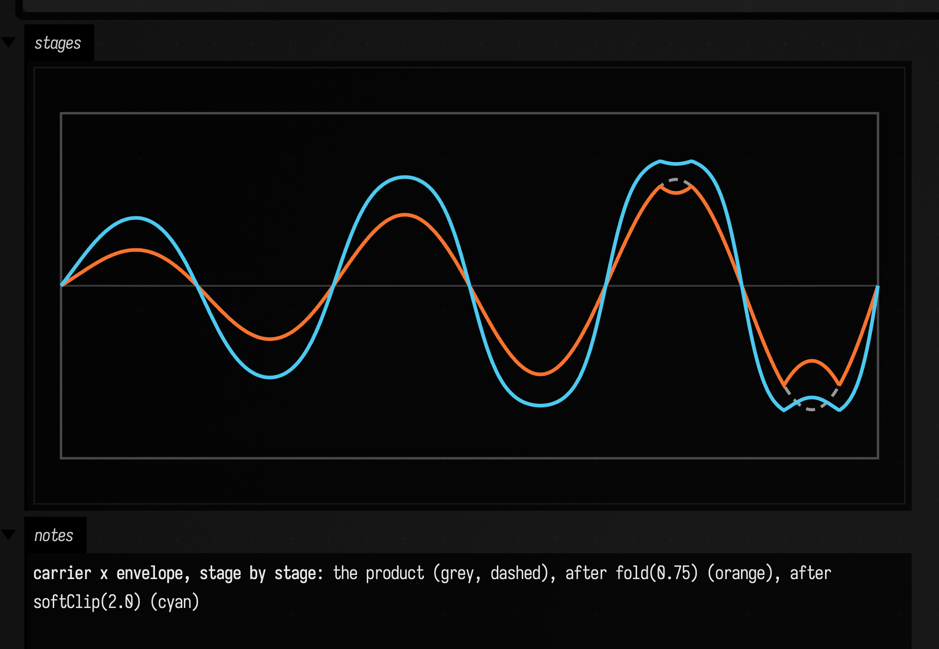
Because every stage returns an Fn, you can plot the pipeline at each stage rather than only at
the end, which is how you find out which stage did the thing you did not want. A tone times an
envelope, then folded, then soft-clipped:
:::static
with(Functions) {
    // One signal, plotted at each stage of its pipeline.
    val carrier = sin(frequency = 3.0, amplitude = 1.0)
    val envelope = ramp(0.2, 1.0) over Functions.Domain.of(0.0, 1.0)
    val stage0 = carrier * envelope
    val stage1 = stage0.fold(0.75)
    val stage2 = stage1.softClip(2.0)

    :::fold the plot frame: 900 x 380 px, y up, values -1.3..1.3
    val x0 = 40.0
    val x1 = 940.0
    val y0 = 30.0
    val y1 = 410.0
    val lo = -1.3
    val hi = 1.3
    val yScale = -(y1 - y0) / (hi - lo)
    val zeroY = y1 + lo * (y1 - y0) / (hi - lo)
    fun curve(fn: Functions.Fn, color: Vec4, thickness: Double, dashed: Boolean = false): List<FLine> {
        val line = fn.toFLine(0.0..1.0, samples = 600, xScale = x1 - x0, yScale = yScale, xOffset = x0, yOffset = zeroY)
        val parts = if (dashed) line.byDashing(10f, 7f) else [line]
        return parts.onEach {
            it.color = color
            it.thickness = thickness
        }
    }
    val guides = [
        fline {
            rect(x0, y0, x1 - x0, y1 - y0)
            color = vec(1.0, 1.0, 1.0, 0.28)
            thickness = 1.6
        },
        fline {
            moveTo(x0, zeroY)
            lineTo(x1, zeroY)
            color = vec(1.0, 1.0, 1.0, 0.30)
            thickness = 1.2
        },
    ]
    val orange = vec(0.97, 0.45, 0.18, 1.0)
    val cyan = vec(0.30, 0.79, 0.94, 1.0)
    val grey = vec(0.6, 0.6, 0.6, 1.0)
    val violet = vec(0.66, 0.50, 0.98, 1.0)
    val green = vec(0.45, 0.85, 0.45, 1.0)
    val pink = vec(0.96, 0.45, 0.72, 1.0)
    :::endfold

    lines(
        guides + curve(stage0, grey, 2.0, dashed = true) + curve(stage1, orange, 2.4) + curve(stage2, cyan, 2.4),
        channel = "stages",
        w = 980.0,
        h = 440.0,
        fitToSize = false,
    )
    markdown(
        "notes",
        "**carrier x envelope, stage by stage**: the product (grey, dashed), after fold(0.75) (orange), " +
            "after softClip(2.0) (cyan)",
    )
}
The editor helps you discover operators
You rarely need to memorise which builders exist. Type an infix operator and a space
(pulseBurst(10) through) and the editor's type-aware infix completion boosts the
operands that fit. Because through (like pipe and /) declares its operand as
FnTransform, every FnTransform-returning builder (gain, delay, lowPass, mirror, …)
floats to the top of the completion list instead of being buried in the alphabetical tail of
everything in scope.
The same help appears after then, which also wants a FnTransform, and it covers any
transform builder you write yourself.
How infix completion finds the operand type
The completion engine reads the operator's declared parameter type by completing the
operator token itself (an infix foo surfaces as foo(ParamType)), then ranks candidates
whose return type matches. See InfixCompletion in
execution.kt.
Once you can build one gesture this way, you can evolve a whole family of them: the
variety-generation section
grows a set of behaviourally distinct shapes from a seed using the same pure-Fn machinery.
Expanded reference: simple + creative patterns
All snippets below assume:
with(Functions) {
    // examples here
}
Unless a snippet says otherwise, functions carry the default domain 0.0..1.0. The periodic family is the exception: sin, cos, saw, triangle, square, pulseTrain, impulseTrain and pulseBurst are built on Domain.ALL, and only narrow an expression when you give them a finite interval.
Most numeric parameters accept plain numbers directly; the DSL lifts them into parameter functions where needed.
Core constructors and base shapes
fn
Use fn when the shape is easiest to write directly as x -> y code over a domain.
Simple
Produces a quadratic curve over the default domain, where each output is x * x.
val f = fn { x -> x * x }Creative
:::static
with(Functions) {
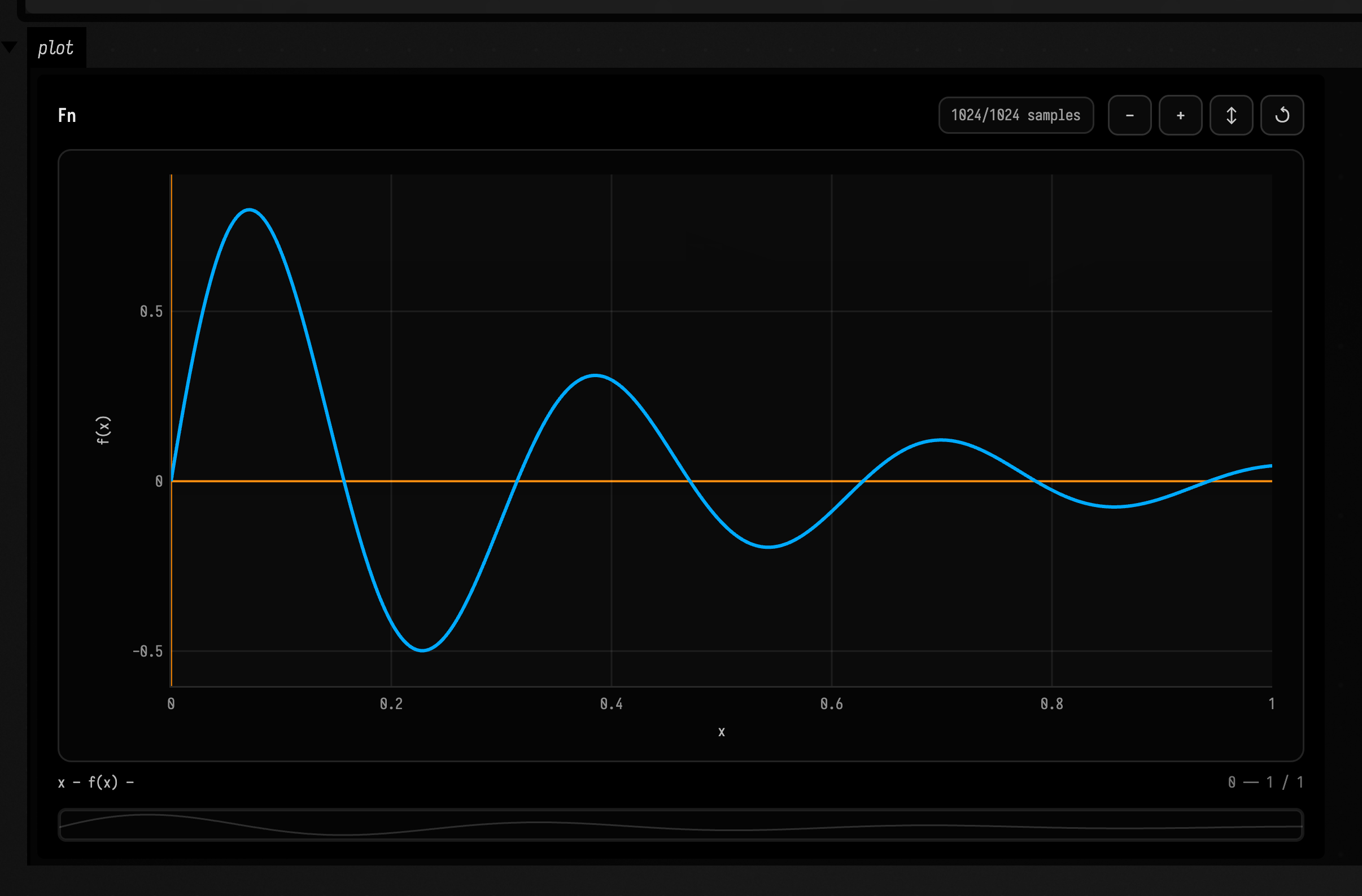
    val f = fn { x -> kotlin.math.sin(20.0 * x) * kotlin.math.exp(-3.0 * x) }
    f.plot()
}
c / constant
Use constants when a scalar needs to participate in Fn arithmetic or carry a domain.
Simple
Produces a flat function that evaluates to 0.5 everywhere in the default domain.
val f = constant(0.5)0.5.c is the same value over Domain.ALL. As a parameter they behave the same, since a constant
never narrows the function it configures: sin(frequency = c(2.0)) and sin(frequency = 2.0.c) are
both unbounded.
Creative
:::static
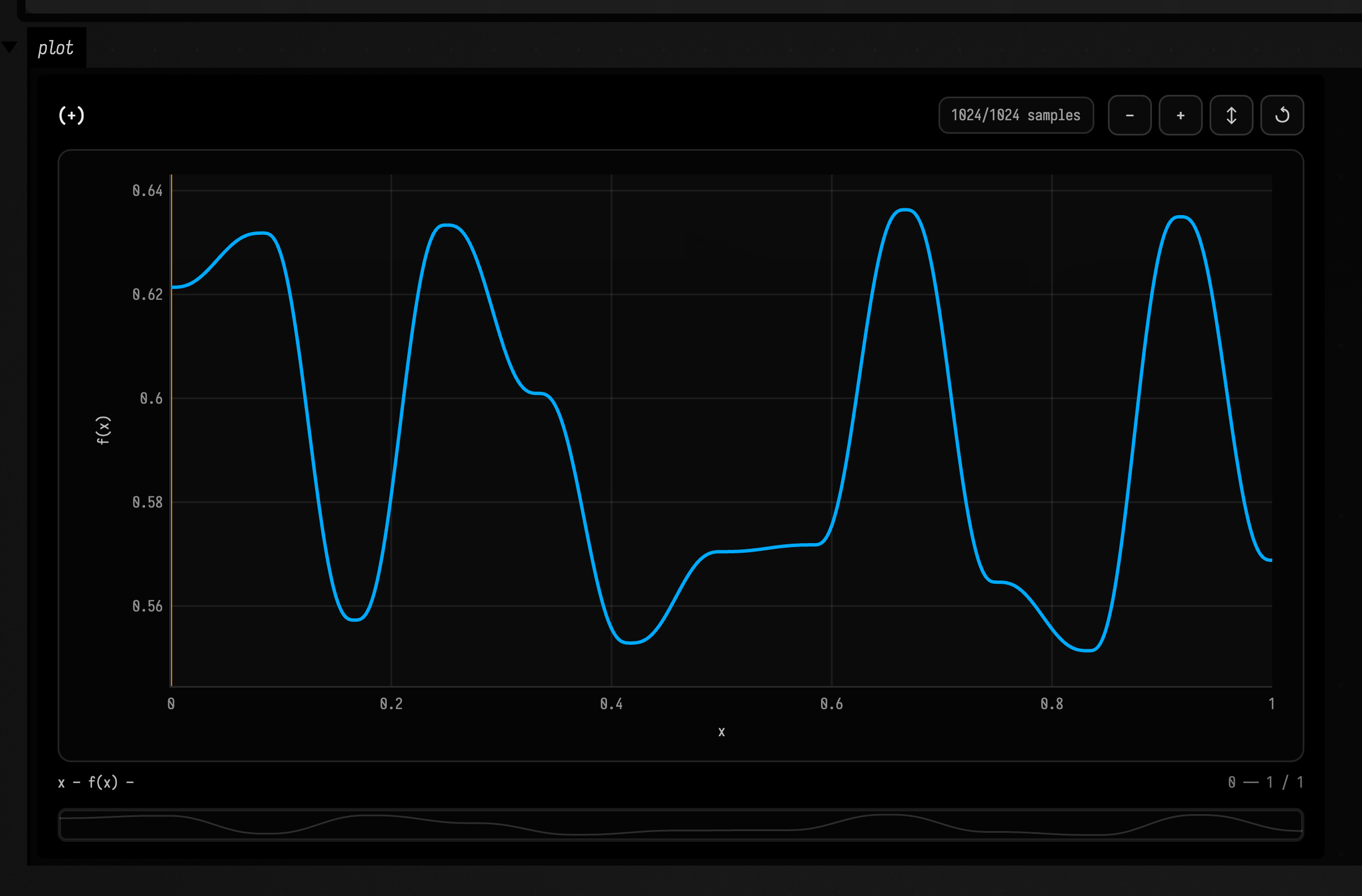
with(Functions) {
    val f = (constant(0.6) + valueNoise(5, 12.0, 0.05)).clamp(0.0, 1.0)
    f.plot()
}
zero / one
zero and one make domain-aware baseline, mask, and gate functions.
Simple
Produces a gate that stays at 1.0 across the whole domain.
val gate = one()Creative
:::static
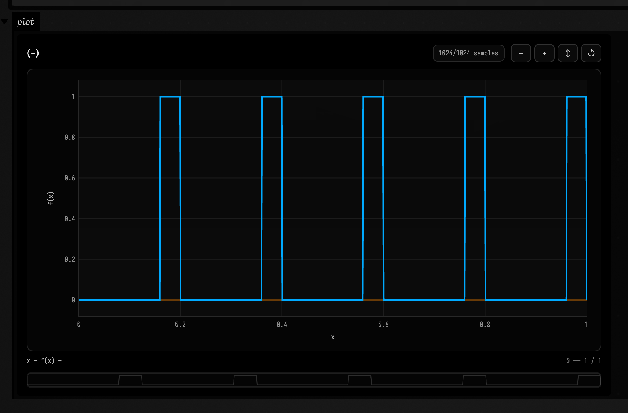
with(Functions) {
    val gate = (one() - pulseTrain(period = 0.2, duty = 0.8)).clip(1.0)
    gate.plot()
}
identity
identity returns the input coordinate, useful as a raw time or normalized-position signal.
Simple
Produces the raw input coordinate as the output value.
val x = identity()Creative
:::static
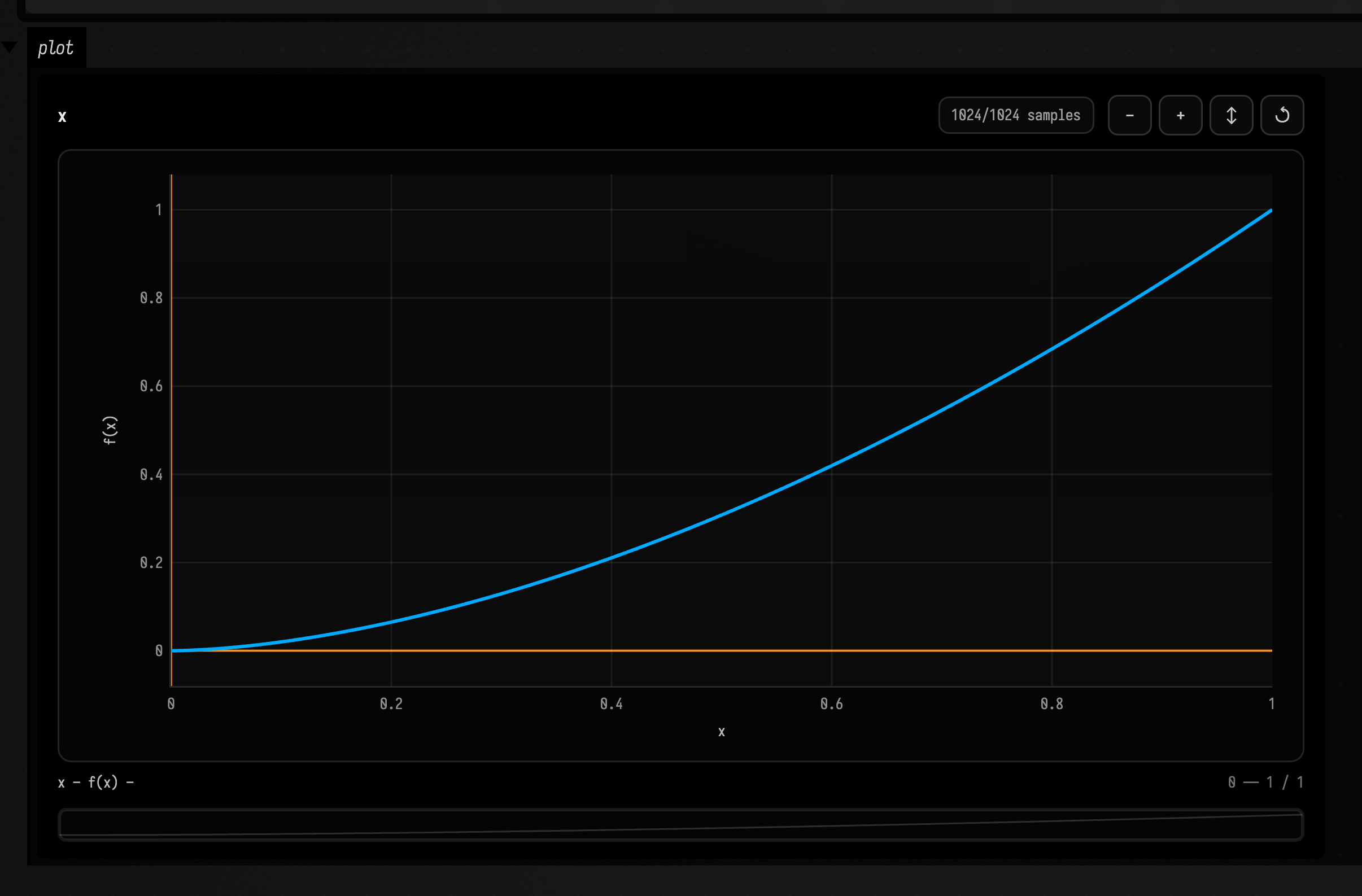
with(Functions) {
    val spiralT = identity().pow(1.7).withEdge(Functions.EdgeMode.CLAMP)
    spiralT.plot()
}
ramp
ramp(start, end) is a value line: its value travels linearly from start to end as x sweeps the domain, so ramp(1.0, 6.0) over (0.0..1.0) is 1 at x=0 and 6 at x=1, and ramp(0.0, 1.0) is the identity 0-to-1 over the default domain. It is the linear sibling of tween, and the go-to for envelopes, selectors, and swept parameters. (To go the other way and normalize an x-window down to 0..1, use remap(from, to), which reads out the position of x within [from, to].)
Simple
Produces a linear 0-to-1 ramp across the default domain.
val r = ramp(0.0, 1.0)Creative
:::static
with(Functions) {
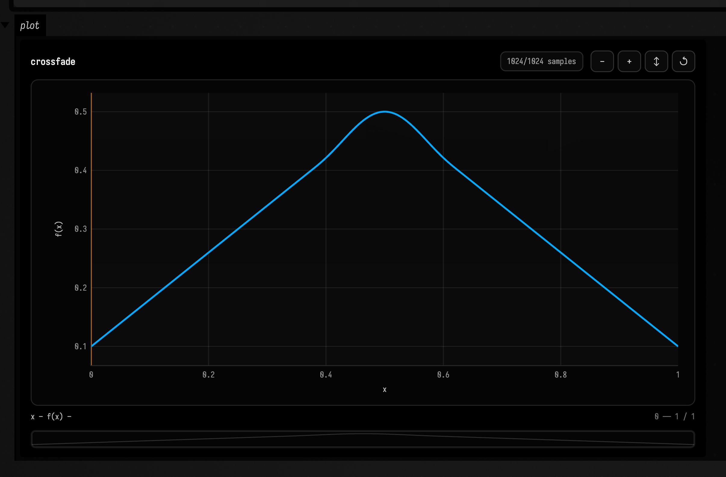
    val env = ramp(0.1, 0.9).crossfade(ramp(0.9, 0.1), center = 0.5, width = 0.25)
    env.plot()
}
step
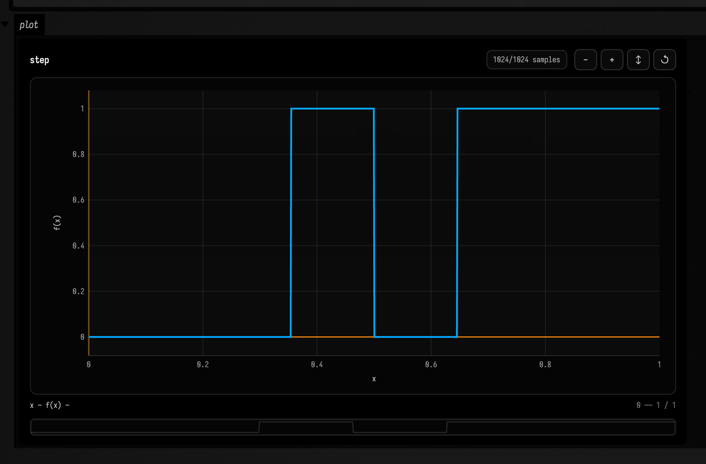
step turns a threshold into a binary gate.
Simple
Produces a hard binary switch at x = 0.5.
val s = step(0.5)Creative
:::static
with(Functions) {
    val trem = step(sin(2.0, amplitude = 0.15, offset = 0.5))
    trem.plot()
}
smoothStep
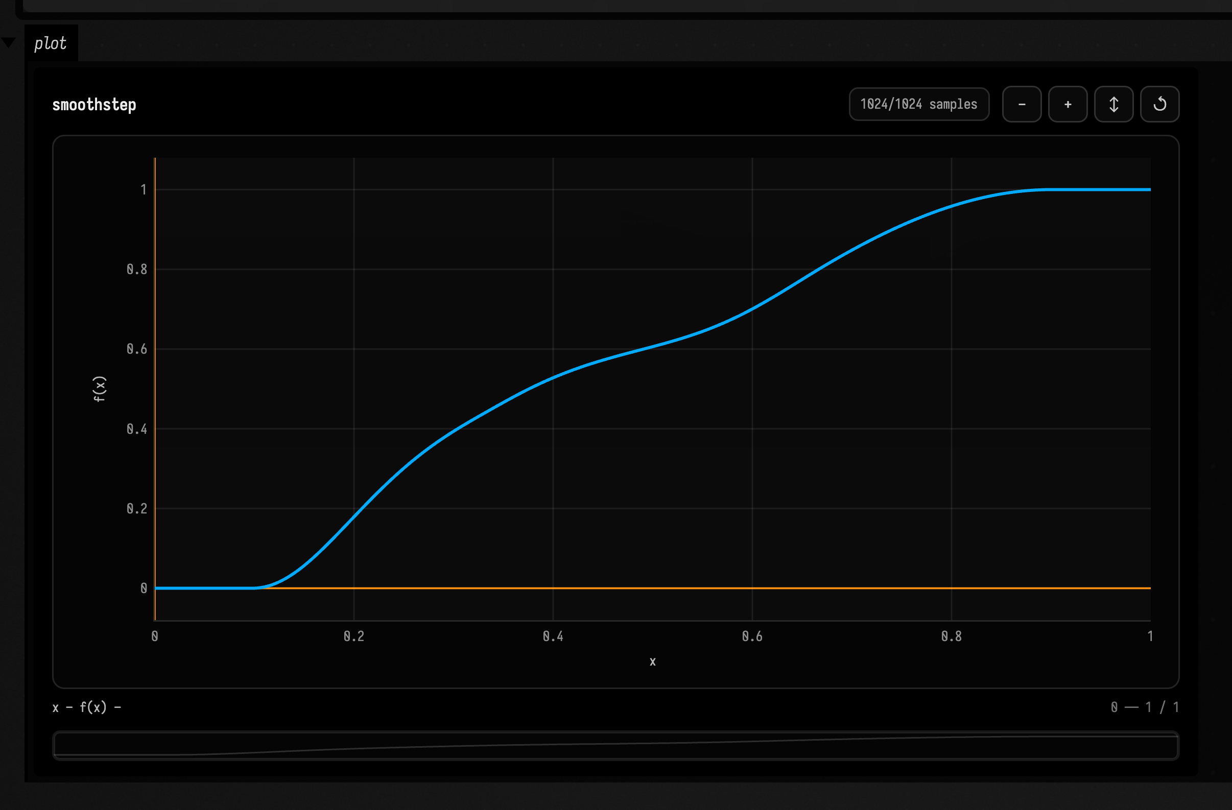
smoothStep turns two edges into a soft 0-to-1 mask.
Simple
Produces a softened 0-to-1 transition between 0.2 and 0.8.
val s = smoothStep(0.2, 0.8)Creative
:::static
with(Functions) {
    val mask = smoothStep(valueNoise(2, 3.0, 0.2), 0.9)
    mask.plot()
}
tween / ease
tween is the direct procedural-animation constructor: it moves between two values (or two Fn signals) across a domain with a named easing curve. Fn.ease(...) shapes an existing normalized signal. Both remain visible and rebuildable in the function graph.
val fade = tween(0.0, 1.0, 2.0..4.0, Functions.Easing.SINE_IN_OUT)
val shapedNoise = valueNoise(3, 4.0, 1.0).ease(Functions.Easing.SMOOTHSTEP)
Easing covers the conventional Penner family, so motion reads the same here as in
other animation toolkits. The polynomial ramps (QUAD, CUBIC, QUART, QUINT),
SINE, EXPO, and CIRC come in _IN, _OUT, and _IN_OUT variants; BACK,
ELASTIC, and BOUNCE add anticipation, spring, and settle; LINEAR,
SMOOTHSTEP, and SMOOTHERSTEP round out the set. A tween clamps normalized time
to its endpoints. ease(..., clampInput = false) is useful when a polynomial shape
should continue beyond 0..1.
Creative
:::static
with(Functions) {
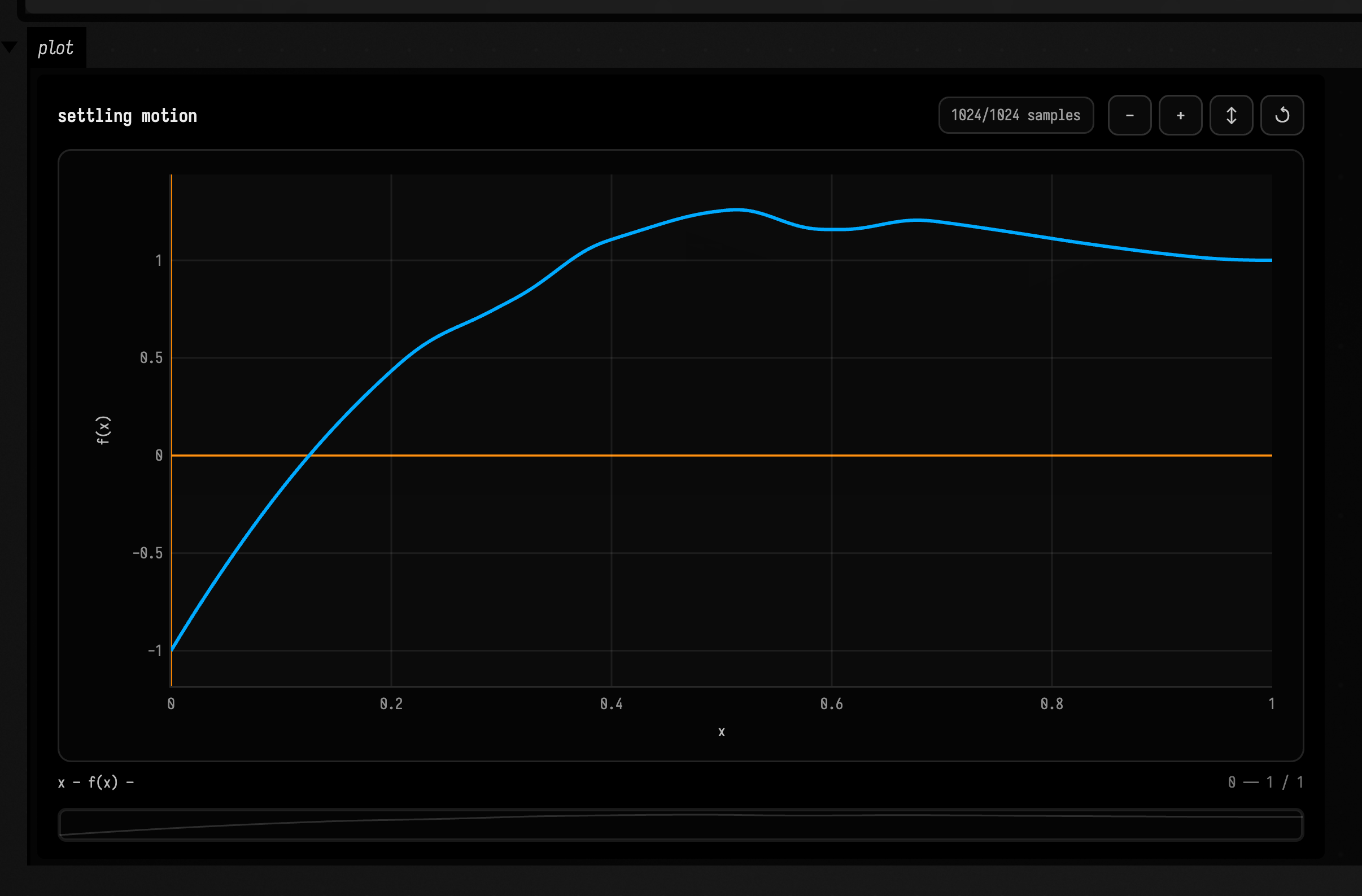
    // A settling spring, textured with a windowed tremor — the headline motion gesture.
    val motion = tween(-1.0, 1.0, 0.0..1.0, Functions.Easing.BACK_OUT)
    val tremor = valueNoise(17, 10.0, 0.08) * hannWindow()
    val texturedMotion = (motion + tremor).withName("settling motion")
    texturedMotion.plot(0.0..1.0)
}
Oscillators and pulse family
sin
sin builds a periodic oscillator from frequency, phase, amplitude, and offset controls.
Simple
Produces a sine wave with three cycles over the unit domain and peak amplitude 0.8.
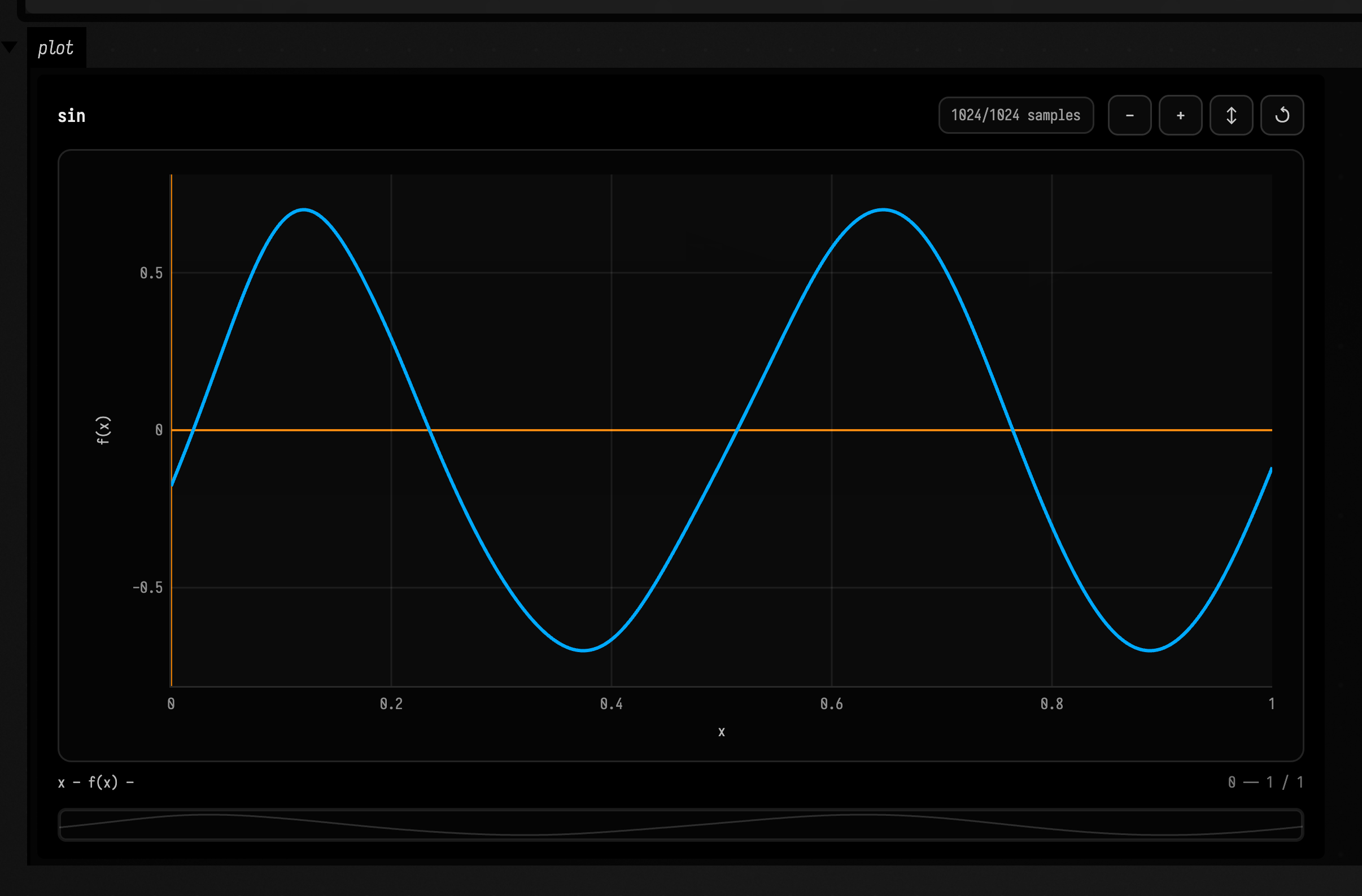
val f = sin(frequency = 3.0, amplitude = 0.8)Creative
:::static
with(Functions) {
    val f = sin(2.0, phase = valueNoise(7, 5.0, 0.3), amplitude = 0.7)
    f.plot()
}
cos
cos is the phase-shifted companion to sin, useful for quadrature and circular motion.
Simple
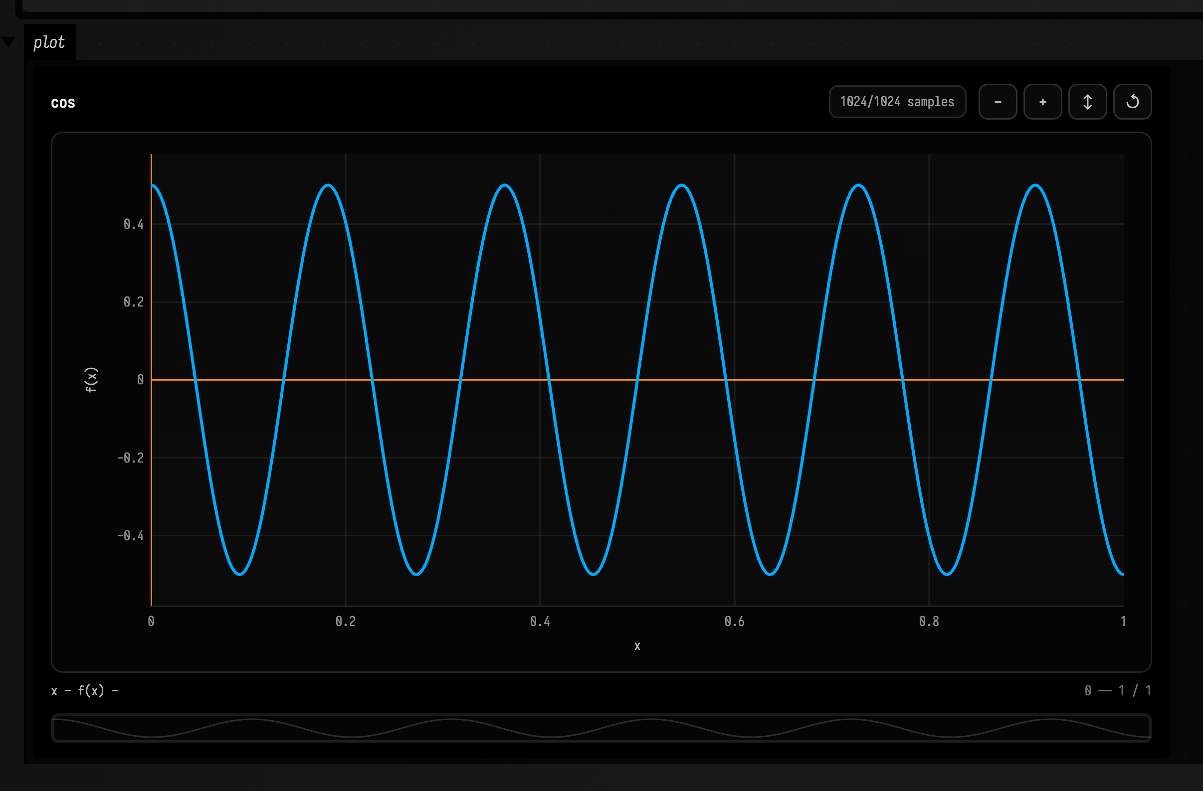
Produces a cosine wave with two cycles and full-scale amplitude.
val f = cos(frequency = 2.0, amplitude = 1.0)Creative
:::static
with(Functions) {
    val f = cos(5.0, phase = ramp(0.0, Math.PI), amplitude = 0.5)
    f.plot()
}
saw
saw creates a repeating ramp with sharp wraparound edges.
Simple
Produces a sawtooth wave that repeats every quarter of the domain.
val f = saw(period = 0.25, amplitude = 1.0)Creative
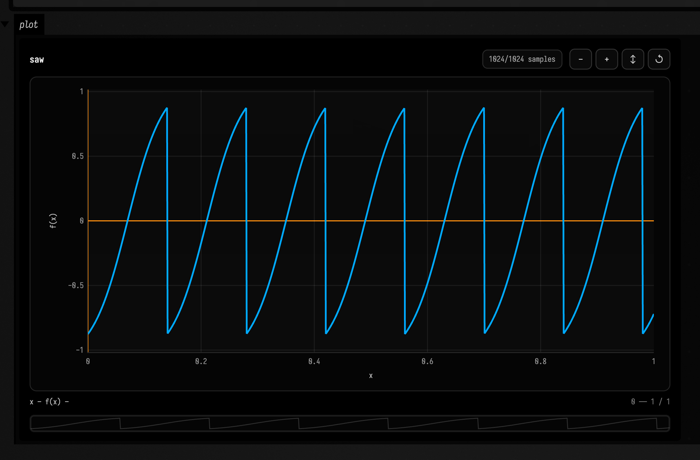
:::static
with(Functions) {
    val f = saw(period = 0.14, amplitude = 0.7).softClip(1.6)
    f.plot()
}
triangle
triangle creates a bipolar linear up/down oscillator.
Simple
Produces a triangle wave with a 0.2 period and 0.9 amplitude.
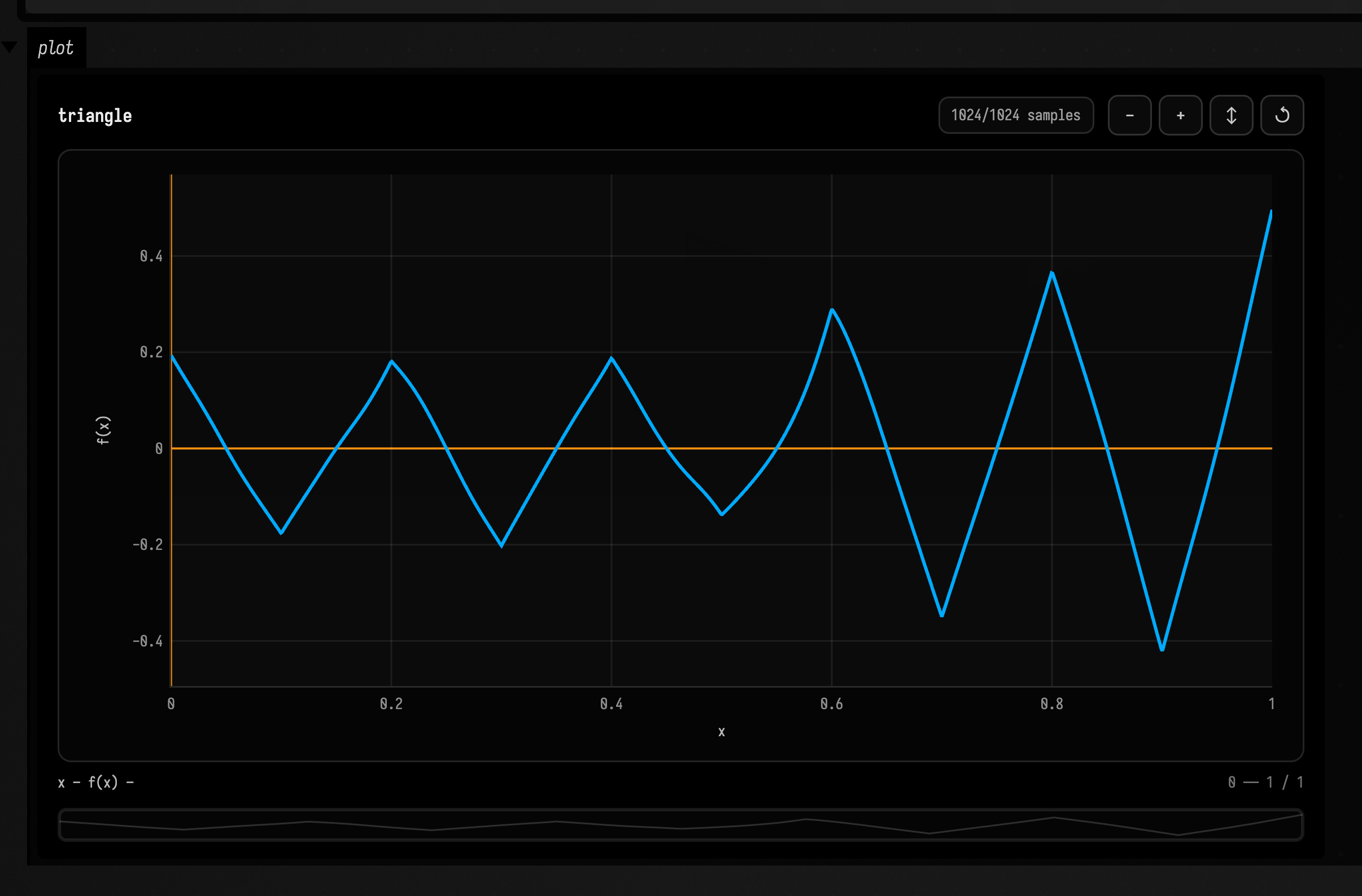
val f = triangle(period = 0.2, amplitude = 0.9)Creative
:::static
with(Functions) {
    val f = triangle(0.2, amplitude = fbm(9, 1.0, 0.6))
    f.plot()
}
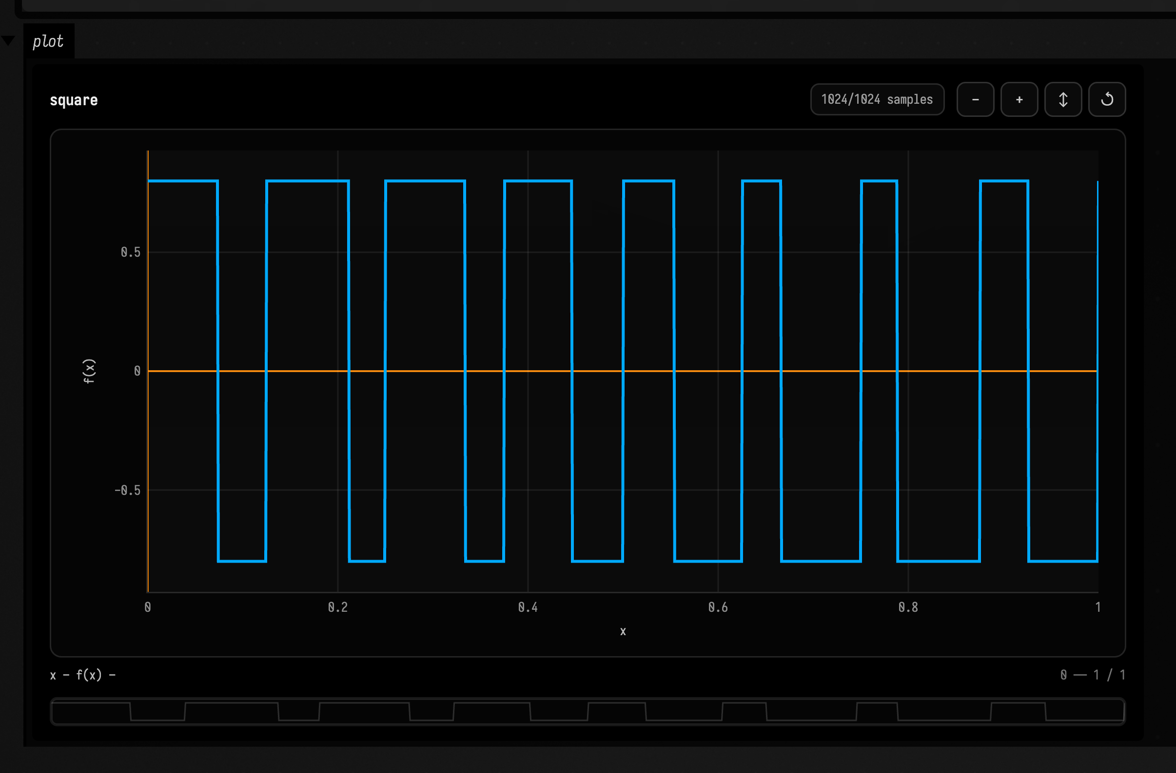
square
square creates a duty-controlled high/low oscillator.
Simple
Produces an even-duty square wave that flips every half-period.
val f = square(period = 0.25, duty = 0.5, amplitude = 1.0)Creative
:::static
with(Functions) {
    val f = square(0.125, duty = sin(1.0, amplitude = 0.2, offset = 0.5), amplitude = 0.8)
    f.plot()
}
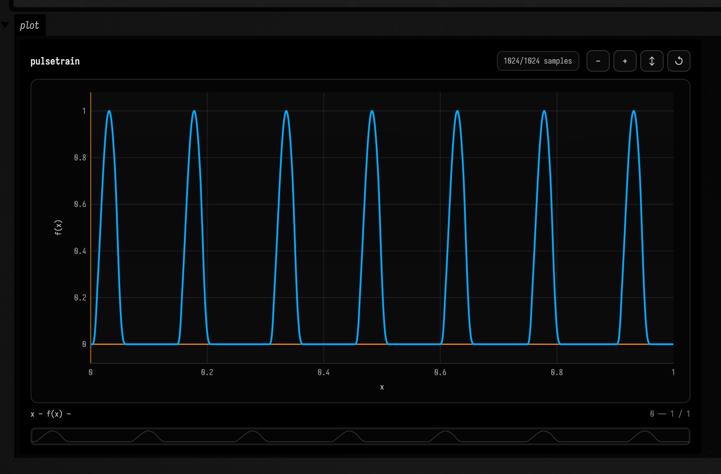
pulseTrain
pulseTrain creates shaped repeating pulses with optional edge, jitter, and profile controls.
Simple
Produces repeating pulses that are high for 35% of each 0.2 period.
val f = pulseTrain(period = 0.2, duty = 0.35)Creative
:::static
with(Functions) {
    val f = pulseTrain(period = 0.15, duty = 0.4, rise = 0.01, fall = 0.02, profile = HANN, jitter = 0.08, seed = 42)
    f.plot()
}
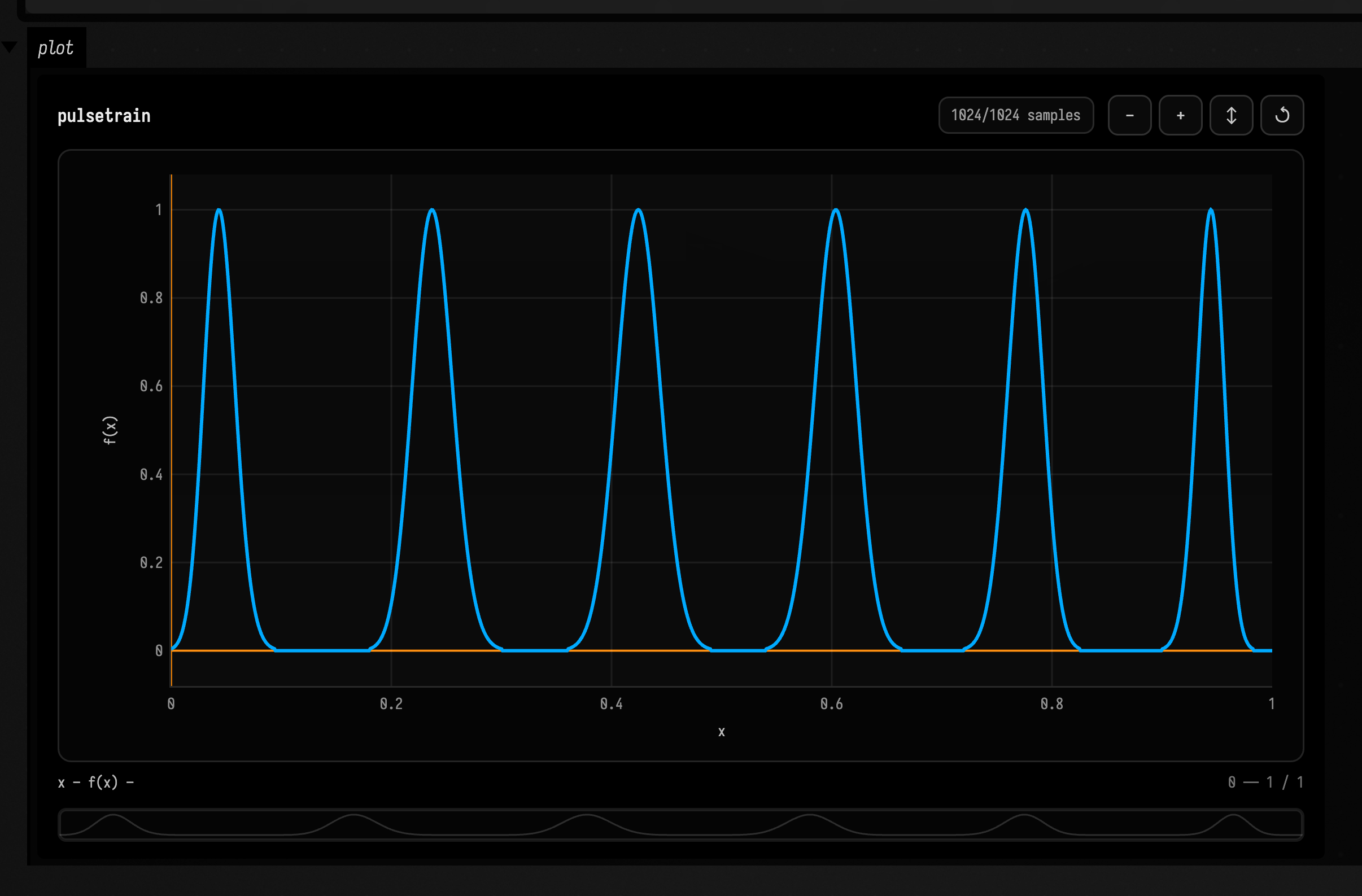
pulseTrainWidth
pulseTrainWidth specifies pulse duration directly instead of duty fraction.
Simple
Produces repeating pulses whose high portion is 0.08 units wide.
val f = pulseTrainWidth(period = 0.2, width = 0.08)Creative
:::static
with(Functions) {
    val f = pulseTrainWidth(period = 0.18, width = sin(0.5, amplitude = 0.05, offset = 0.08), profile = GAUSSIAN)
    f.plot()
}
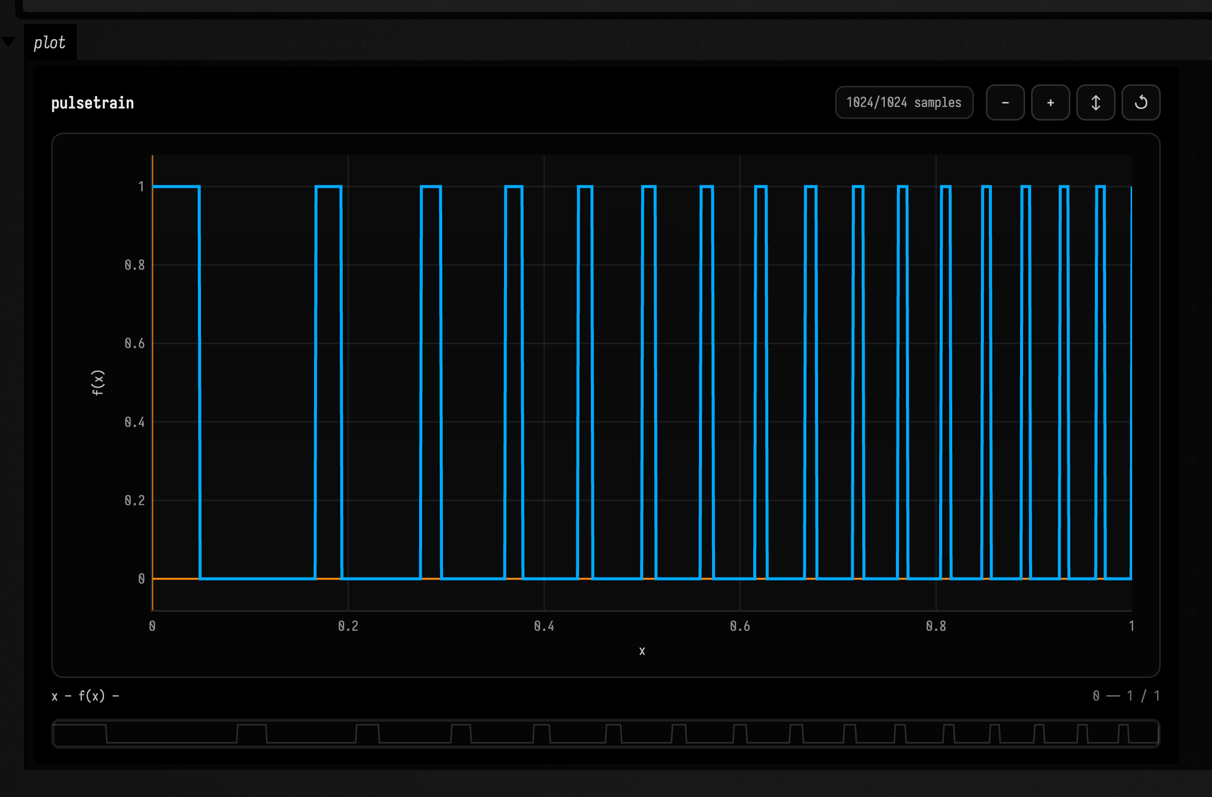
pulseTrainHz
pulseTrainHz describes pulses by frequency instead of period.
Simple
Produces eight pulses per unit, with each pulse high for 30% of its cycle.
val f = pulseTrainHz(frequency = 8.0, duty = 0.3)Creative
:::static
with(Functions) {
    val f = pulseTrainHz(frequency = ramp(4.0, 16.0), duty = 0.22, edge = Functions.PulseEdge.SINE)
    f.plot()
}
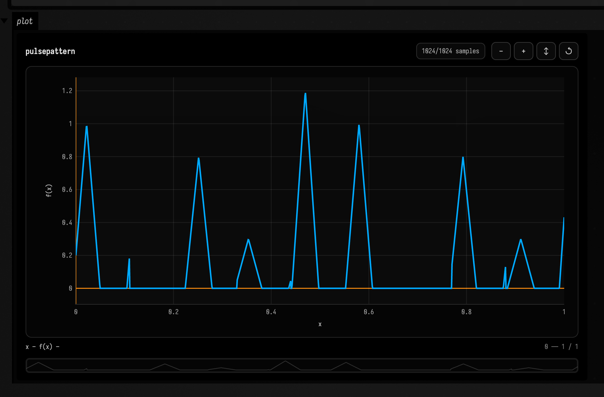
pulseTrainPattern
pulseTrainPattern cycles through per-pulse amplitudes for rhythmic patterns.
Simple
Produces a pulse train whose pulse heights cycle through the supplied pattern.
val f = pulseTrainPattern(doubleArrayOf(1.0, 0.5, 1.0, 0.2), period = 0.2)Creative
:::static
with(Functions) {
    val f = pulseTrainPattern(doubleArrayOf(1.0, 0.0, 0.8, 0.3, 1.2), period = 0.11, jitter = 0.1, profile = TRIANGLE)
    f.plot()
}
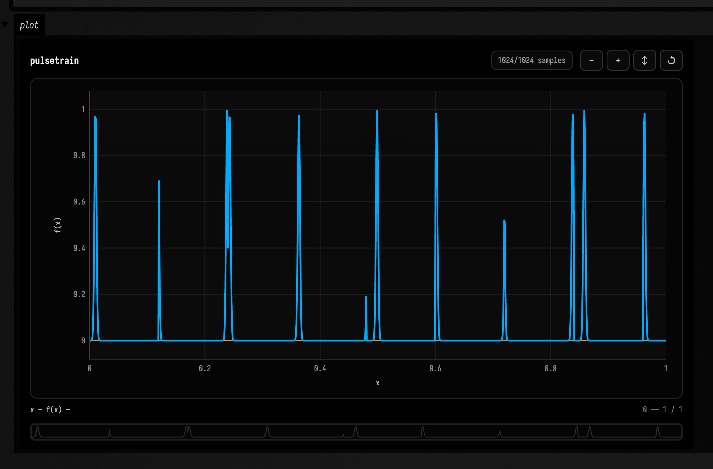
impulseTrain
impulseTrain makes narrow Gaussian-style events at a repeating period.
Simple
Produces narrow repeating impulses every 0.1 units.
val f = impulseTrain(period = 0.1, width = 0.01)Creative
:::static
with(Functions) {
    val f = impulseTrain(period = 0.12, width = 0.02, sigma = 0.09, jitter = 0.2, seed = 9)
    f.plot()
}
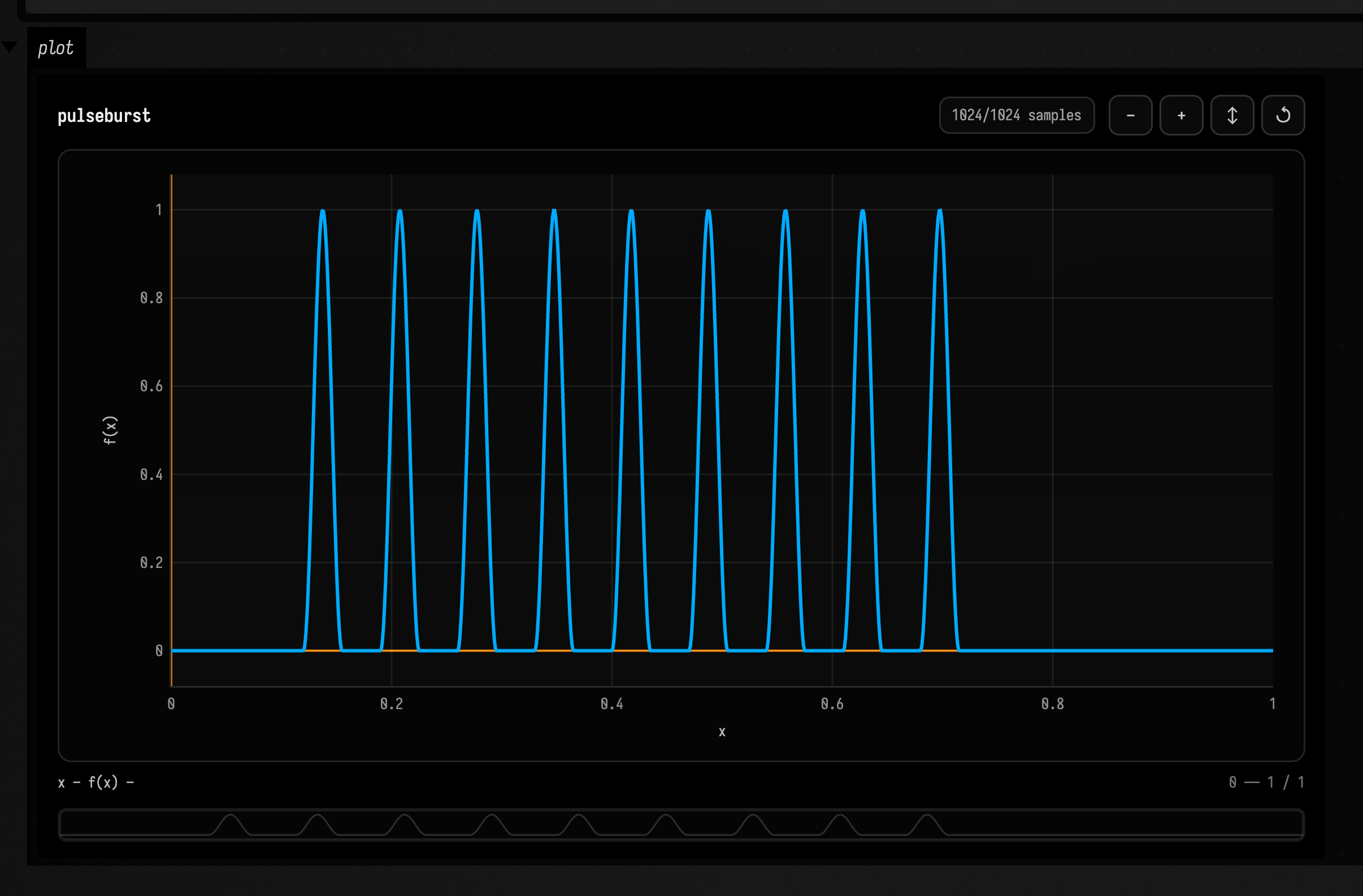
pulseBurst
pulseBurst limits a pulse train to a finite count of events.
Simple
Produces five short pulses starting at 0.2 and spaced by 0.1.
val f = pulseBurst(count = 5, period = 0.1, start = 0.2)Creative
:::static
with(Functions) {
    val f = pulseBurst(9, period = 0.07, start = 0.12, edge = EXP, curve = 3.0, profile = HANN)
    f.plot()
}
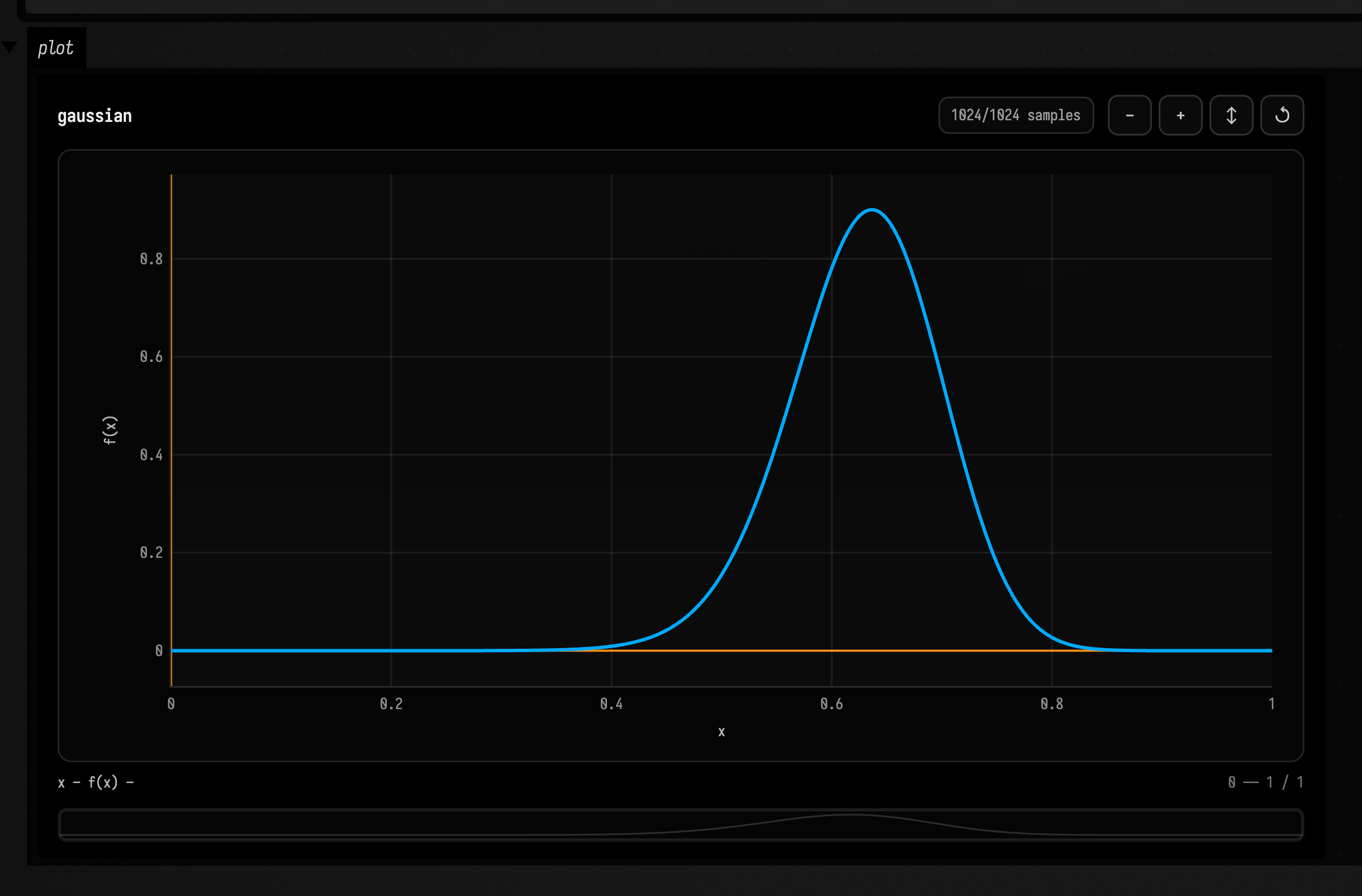
gaussian
gaussian makes a bell-shaped lobe that can be used as an envelope, bump, or mask.
Simple
Produces a unit Gaussian bump centered at 0.5 with 0.1 spread.
val f = gaussian(mean = 0.5, sigma = 0.1, amplitude = 1.0)Creative
:::static
with(Functions) {
    val f = gaussian(mean = sin(0.5, amplitude = 0.15, offset = 0.5), sigma = 0.08, amplitude = 0.9)
    f.plot()
}
Algebra and mapping
+ - * /
Arithmetic combines functions pointwise, intersecting domains where both inputs are valid.
Simple
Produces the pointwise sum of a sine wave and a sawtooth wave.
val f = sin(2.0) + saw(0.2)Creative
:::static
with(Functions) {
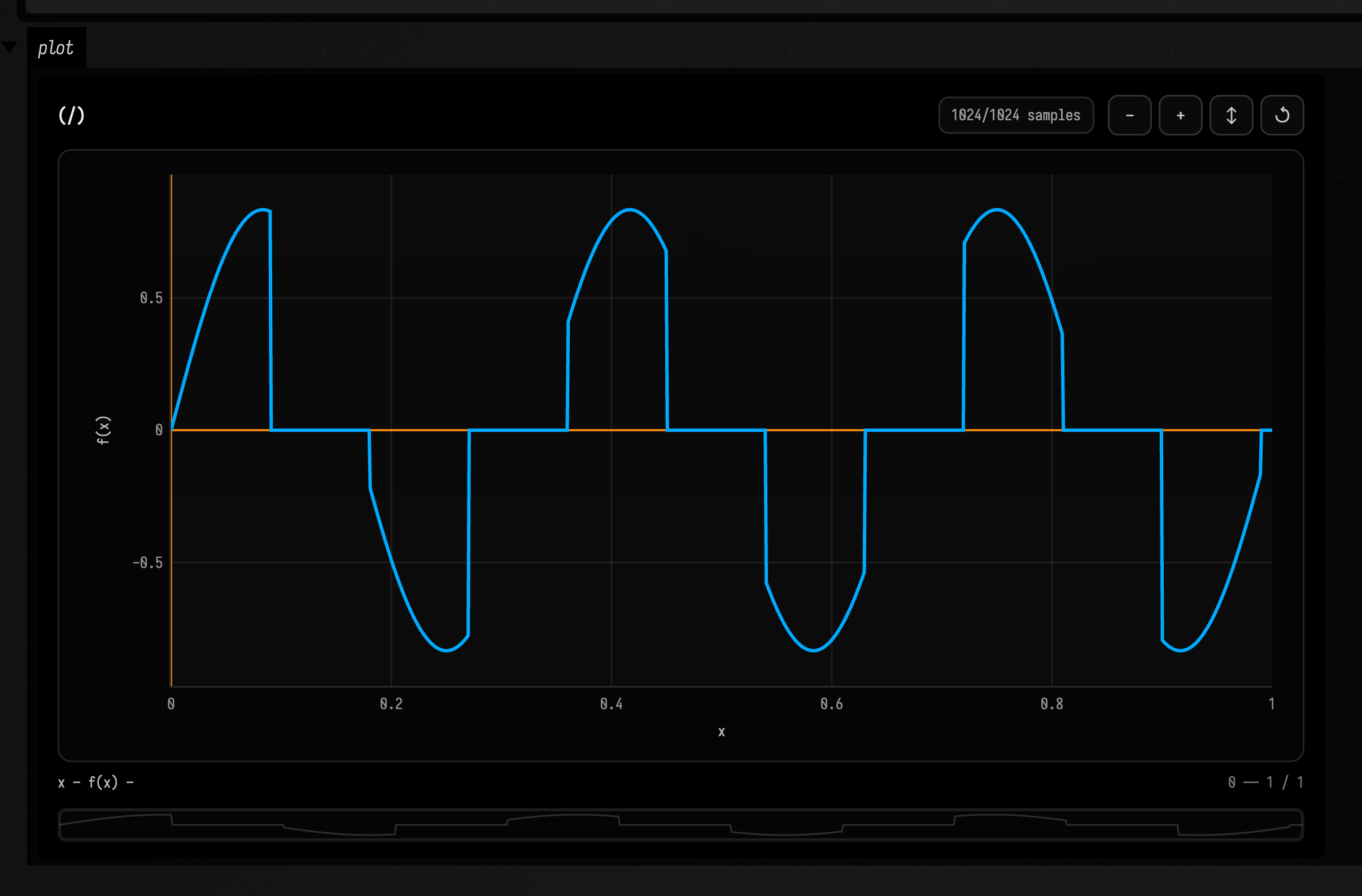
    val f = (sin(3.0) * pulseTrain(0.18)) / (one() + constant(0.2))
    f.plot()
}
mapY
mapY reshapes output values while leaving time alone.
Simple
Halves the sine wave's output values without changing its timing.
val f = sin(2.0).mapY { it * 0.5 }Creative
:::static
with(Functions) {
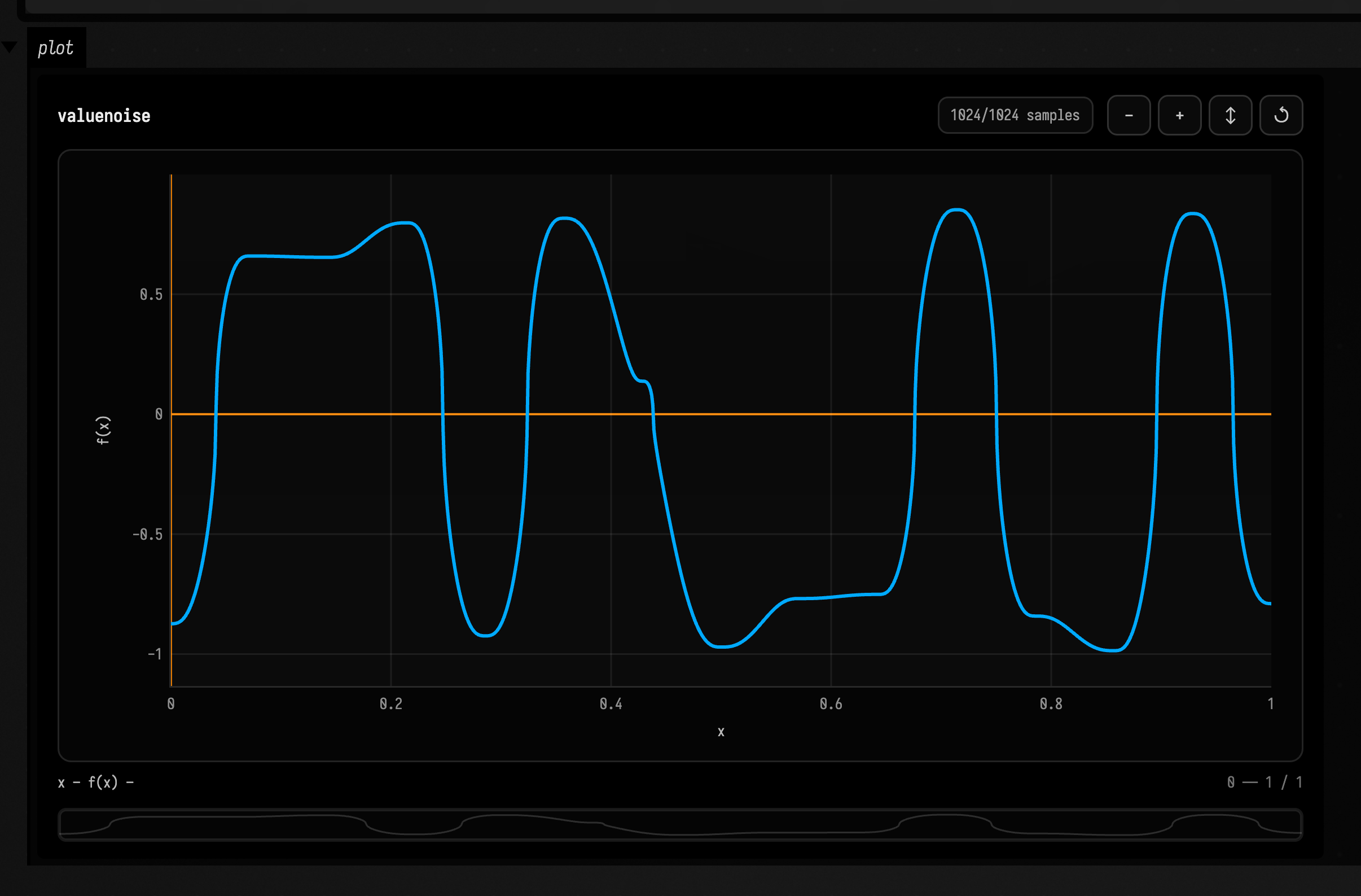
    val f = valueNoise(3, 14.0, 1.0).mapY { v -> kotlin.math.sign(v) * kotlin.math.sqrt(kotlin.math.abs(v)) }
    f.plot()
}
mapX
mapX warps the input coordinate before sampling the source function.
Simple
Stretches the sine wave horizontally by sampling it at half the input coordinate.
val f = sin(2.0).mapX { x -> x * 0.5 }Creative
:::static
with(Functions) {
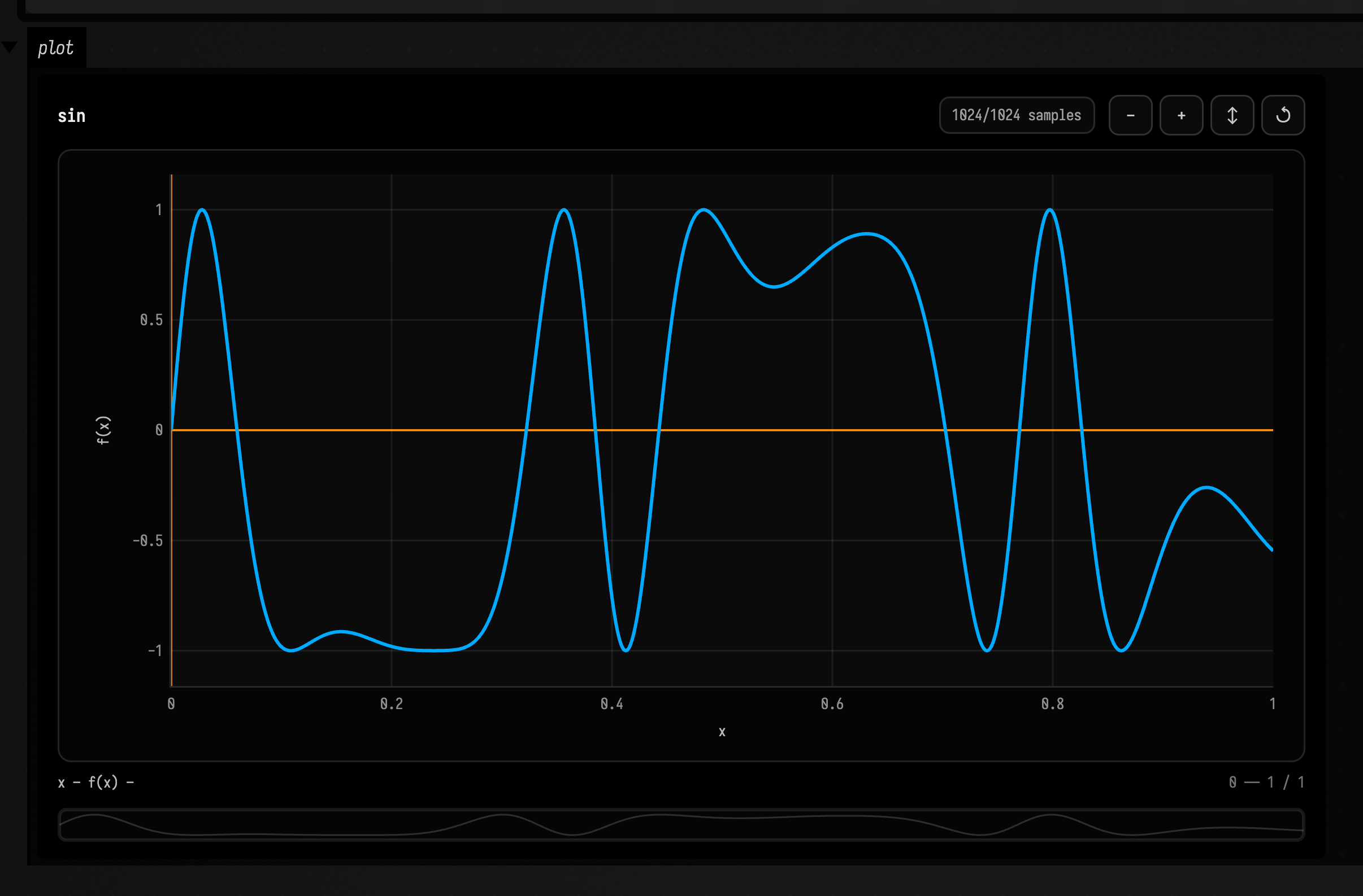
    val f = sin(4.0).mapX { x -> x + 0.08 * kotlin.math.sin(16.0 * x) }
    f.plot()
}
shift / delay
shift and delay sample the source earlier or later in x.
Simple
Moves the sine wave forward in time by 0.1 units.
val f = sin(2.0).shift(0.1)Creative
:::static
with(Functions) {
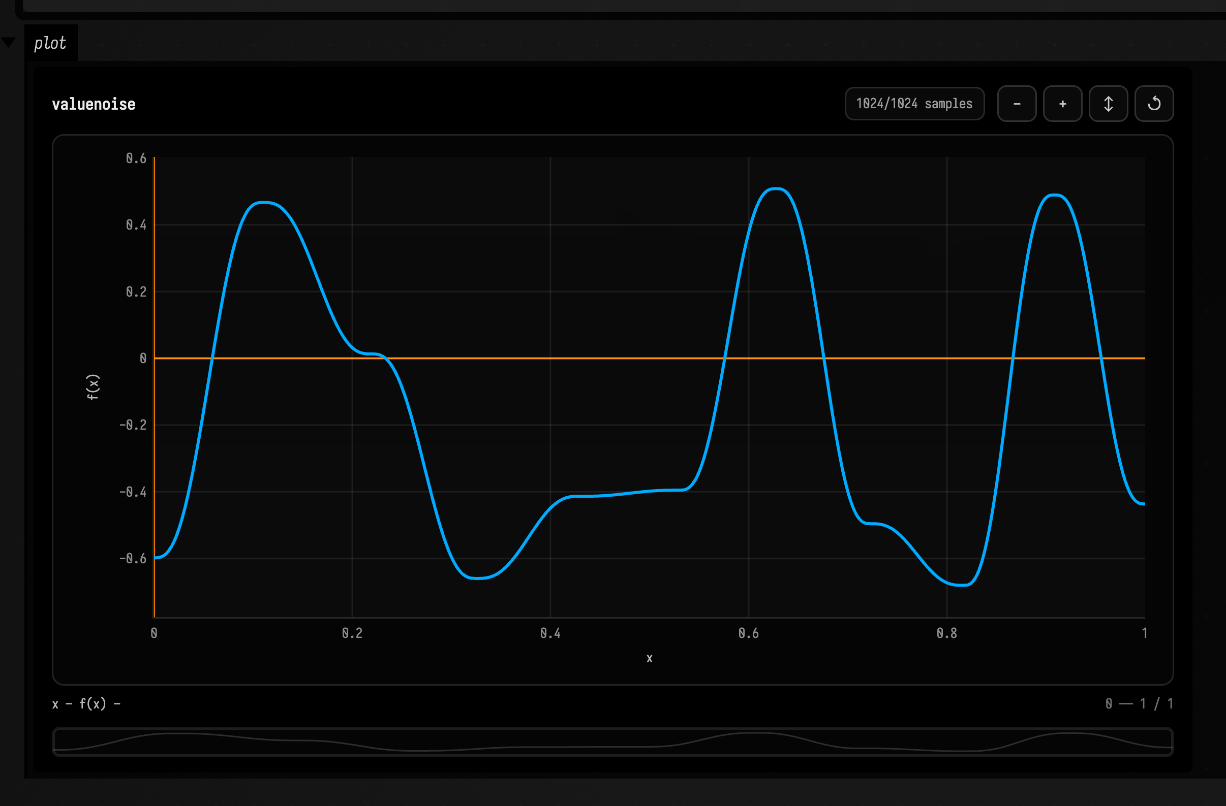
    val f = valueNoise(7, 10.0, 0.7).delay(sin(0.5, amplitude = 0.03))
    f.plot()
}
scaleX / faster / slower
Time-scaling changes how quickly the source is traversed.
Simple
Stretches the saw wave's time axis by a factor of two.
val f = saw(0.2).scaleX(2.0)Creative
:::static
with(Functions) {
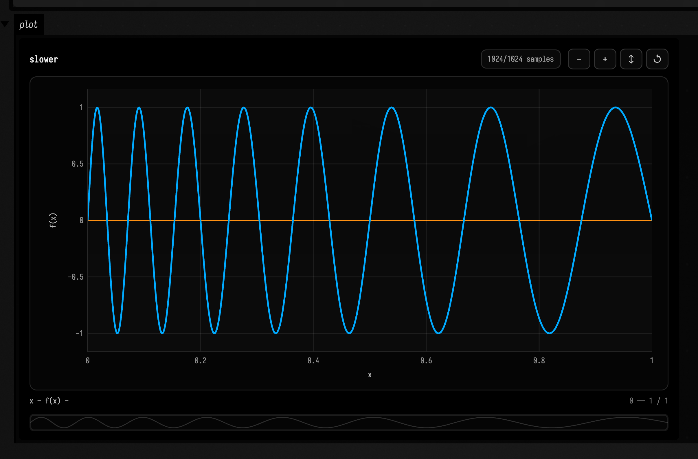
    val f = (sin(3.0).faster(2.0) / slower(0.75)).scaleX(scale = ramp(0.8, 1.6), about = 0.5)
    f.plot()
}
scaleY / offsetY
Y-scaling and offsetting change the amplitude range without moving events in time.
Simple
Halves the sine wave's amplitude and lifts it upward by 0.2.
val f = sin(2.0).scaleY(0.5).offsetY(0.2)Creative
:::static
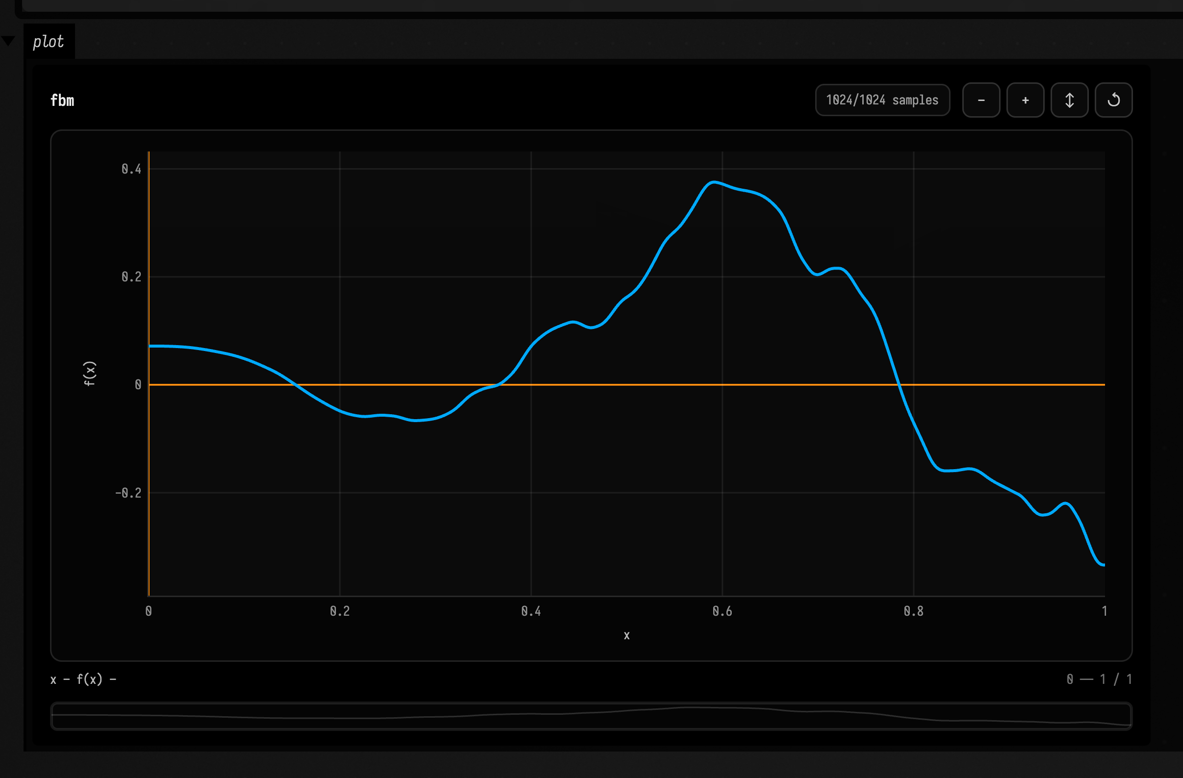
with(Functions) {
    val f = fbm(1, 2.0, 1.0).scaleY(smoothStep(0.0, 1.0)).offsetY(valueNoise(2, 3.0, 0.1))
    f.plot()
}
reverse / flip
Reverse mirrors time around a point, while flip negates the output.
Simple
Reverses the ramp so it falls from one to zero across the domain.
val f = ramp(0.0, 1.0).reverse()Creative
:::static
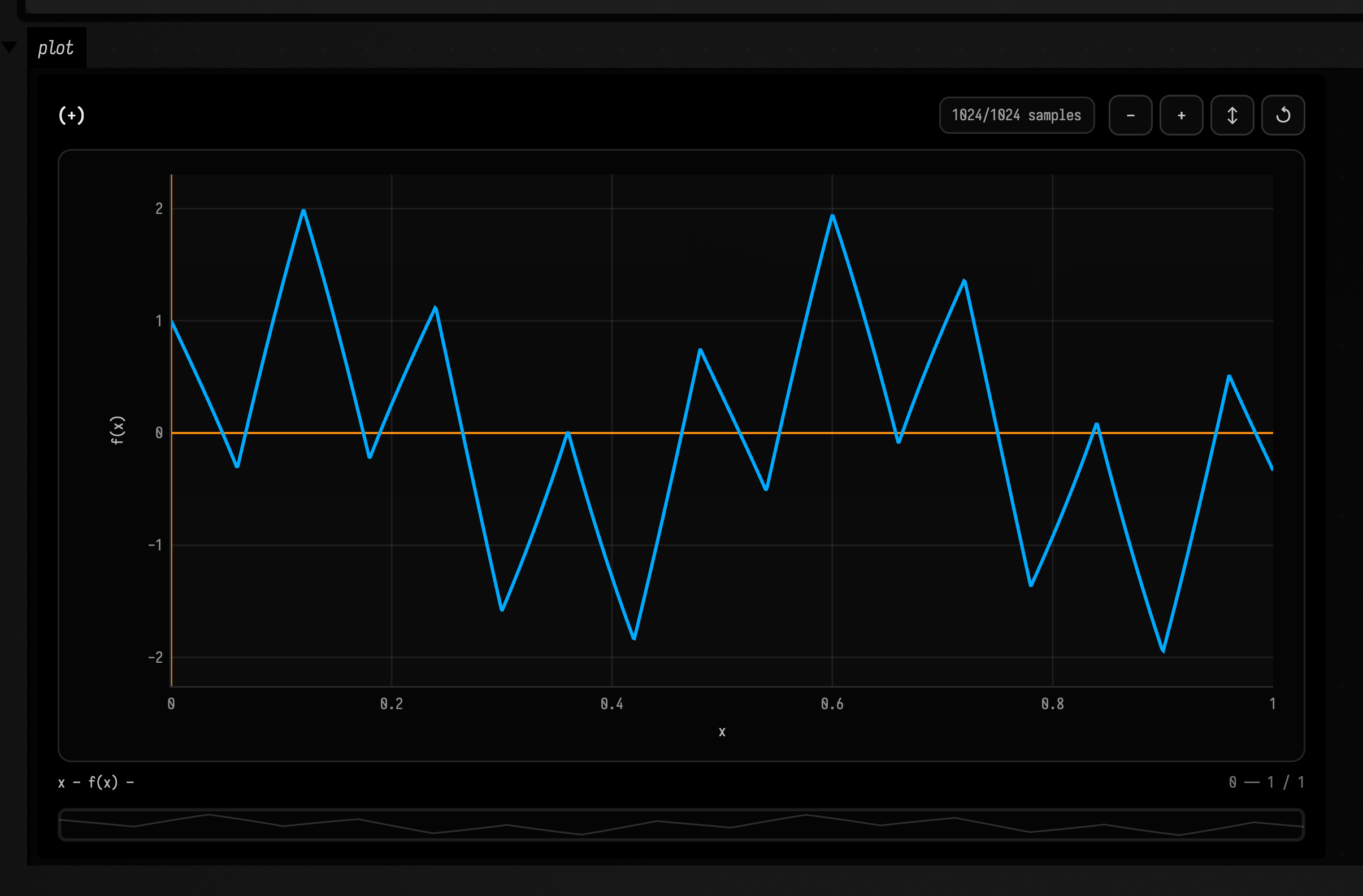
with(Functions) {
    val f = (sin(2.0).reverse(0.5) + triangle(0.12)).flip()
    f.plot()
}
abs / sign / rectify
These turn bipolar signals into magnitude, sign, or positive-only shapes.
Simple
Folds negative sine values upward into positive values.
val f = sin(3.0).abs()Creative
:::static
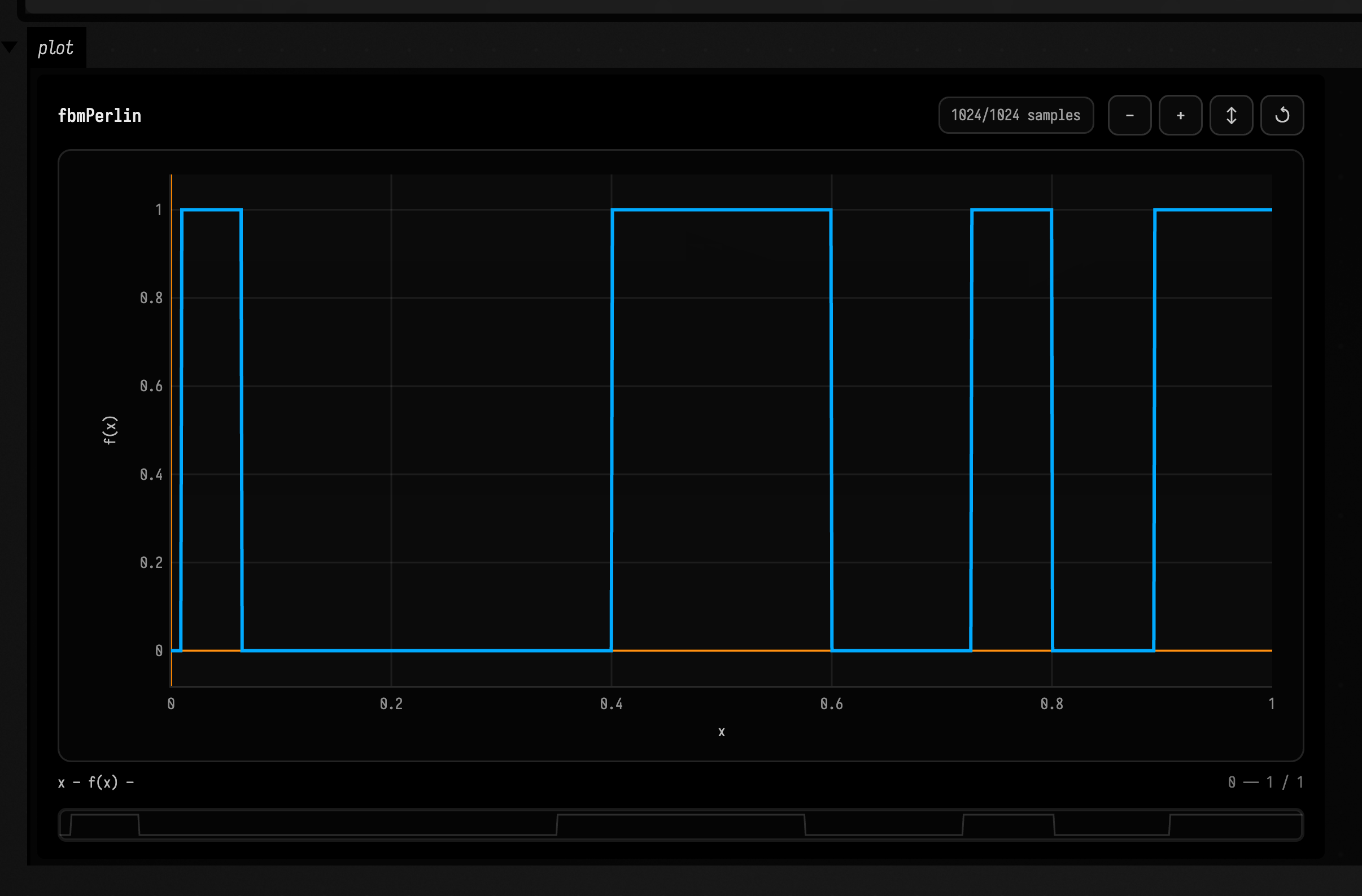
with(Functions) {
    val f = fbmPerlin(7, 2.5, 1.0).sign().rectify()
    f.plot()
}
pow / exp / log
Power and logarithmic transforms bend a signal curve nonlinearly.
Simple
Squares the linear ramp, bending it into an ease-in curve.
val f = ramp(0.0, 1.0).pow(2.0)Creative
:::static
with(Functions) {
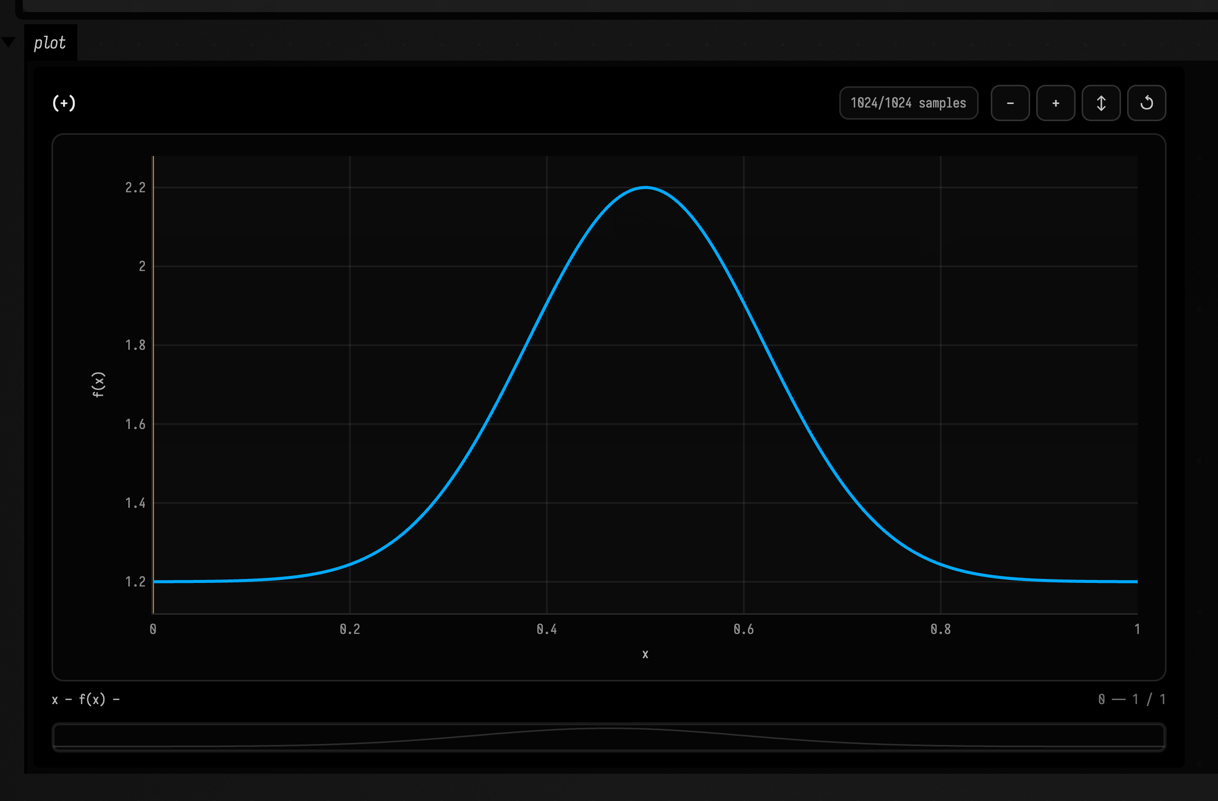
    val f = (gaussian(0.5, 0.12, 1.0) + constant(1.2)).log(kotlin.math.E).exp()
    f.plot()
}
clamp / clip / softClip / fold / wrapY
Limiters and wrappers keep outputs in a usable range, either gently or with hard edges.
Simple
Limits the sine wave so values never exceed 0.7 in magnitude.
val f = sin(2.0).clip(0.7)Creative
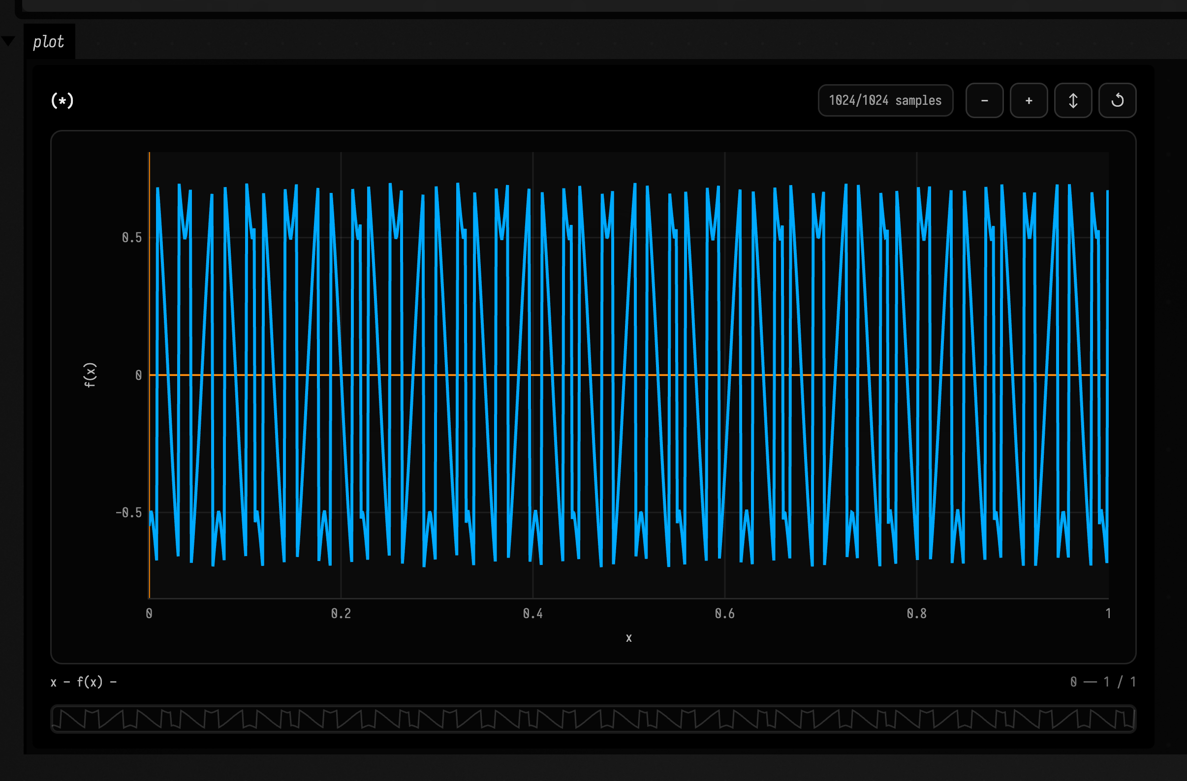
:::static
with(Functions) {
    val f = (saw(0.11) * constant(2.5)).fold(0.8).softClip(1.4).wrapY(-0.7, 0.7)
    f.plot()
}
withEdge
withEdge defines how a function behaves when sampled outside its domain.
Simple
Makes out-of-domain samples clamp to the nearest edge value.
val f = sin(3.0).withEdge(Functions.EdgeMode.CLAMP)Creative
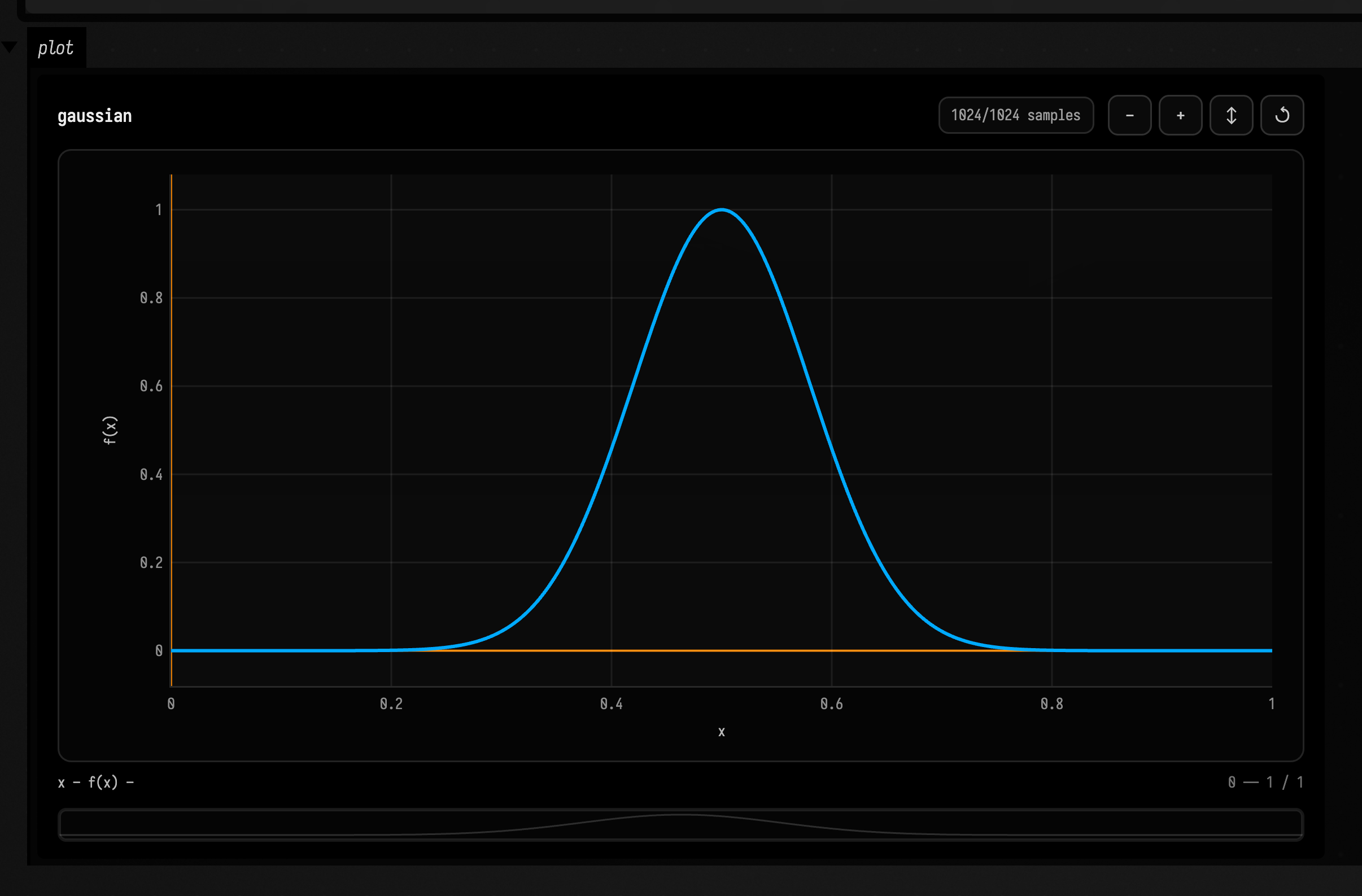
:::static
with(Functions) {
    val f = gaussian(0.5, 0.08, 1.0).withEdge(Functions.EdgeMode.MIRROR, outside = valueNoise(8, 4.0, 0.05))
    f.plot()
}
quantize / bitCrush
Quantizers reduce continuous values into stepped or bit-depth-like levels.
Simple
Reduces the sine wave to eight discrete value levels.
val f = sin(2.0).quantize(8)Creative
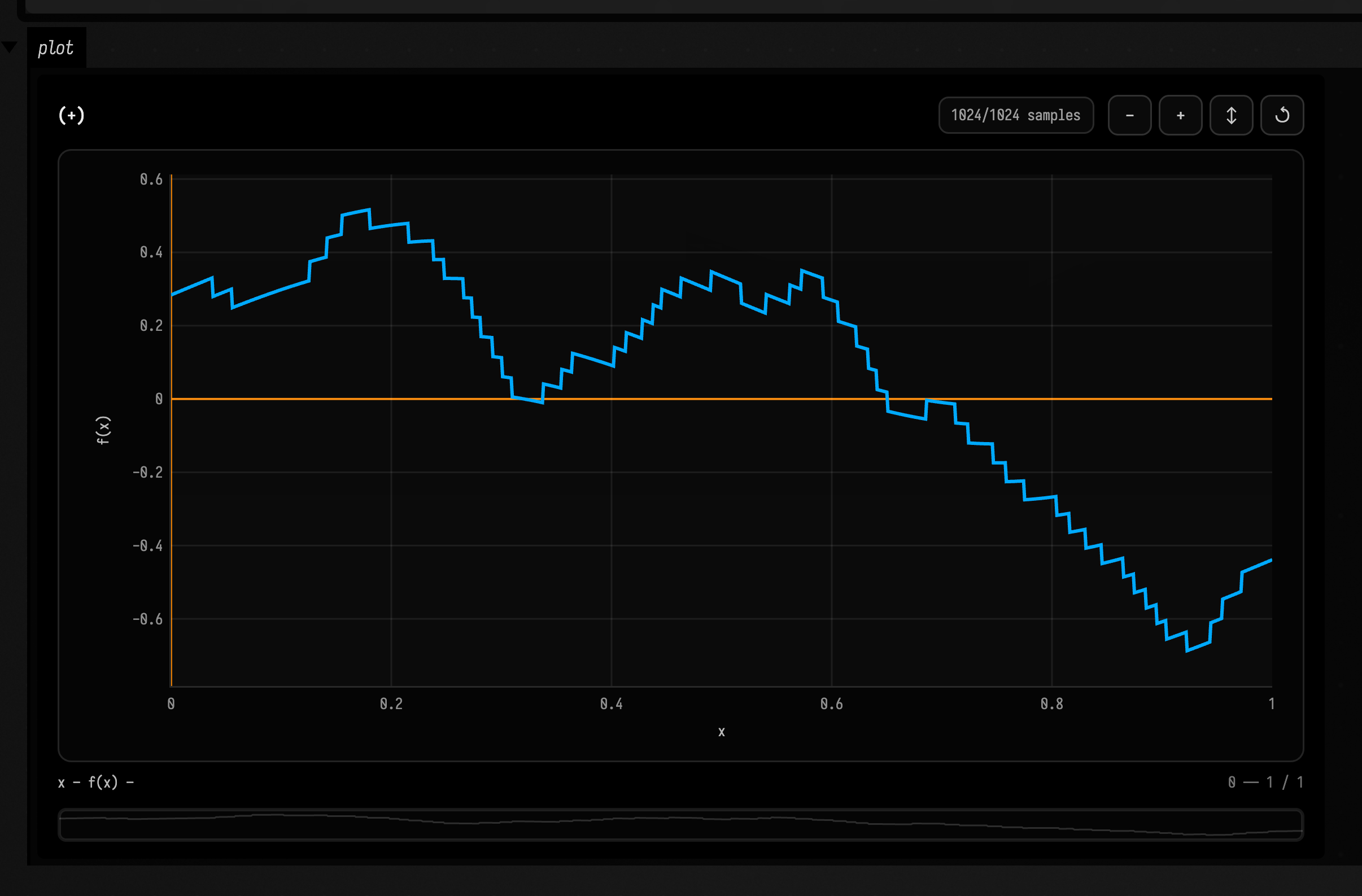
:::static
with(Functions) {
    val f = (fbm(4, 3.0, 1.0).bitCrush(5)).mix(sin(1.0), constant(0.2))
    f.plot()
}
mix / crossfade
Mixing blends between functions, either by a fixed amount or over a transition region.
Simple
Blends halfway between the sine and saw waves.
val f = sin(2.0).mix(saw(0.2), 0.5)Creative
:::static
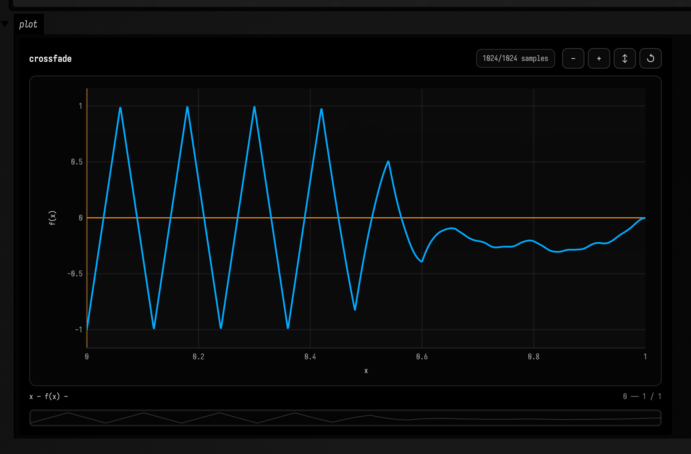
with(Functions) {
    val f = triangle(0.12).crossfade(fbmPerlin(11, 2.0, 1.0), center = 0.55, width = 0.35)
    f.plot()
}
cut / trim / slice / replace
Interval edits keep or swap parts of a function over a target range.
Simple
Keeps only the 0.2..0.8 portion of the sine wave as the function's domain.
val f = sin(2.0).cut(0.2..0.8)Creative
:::static
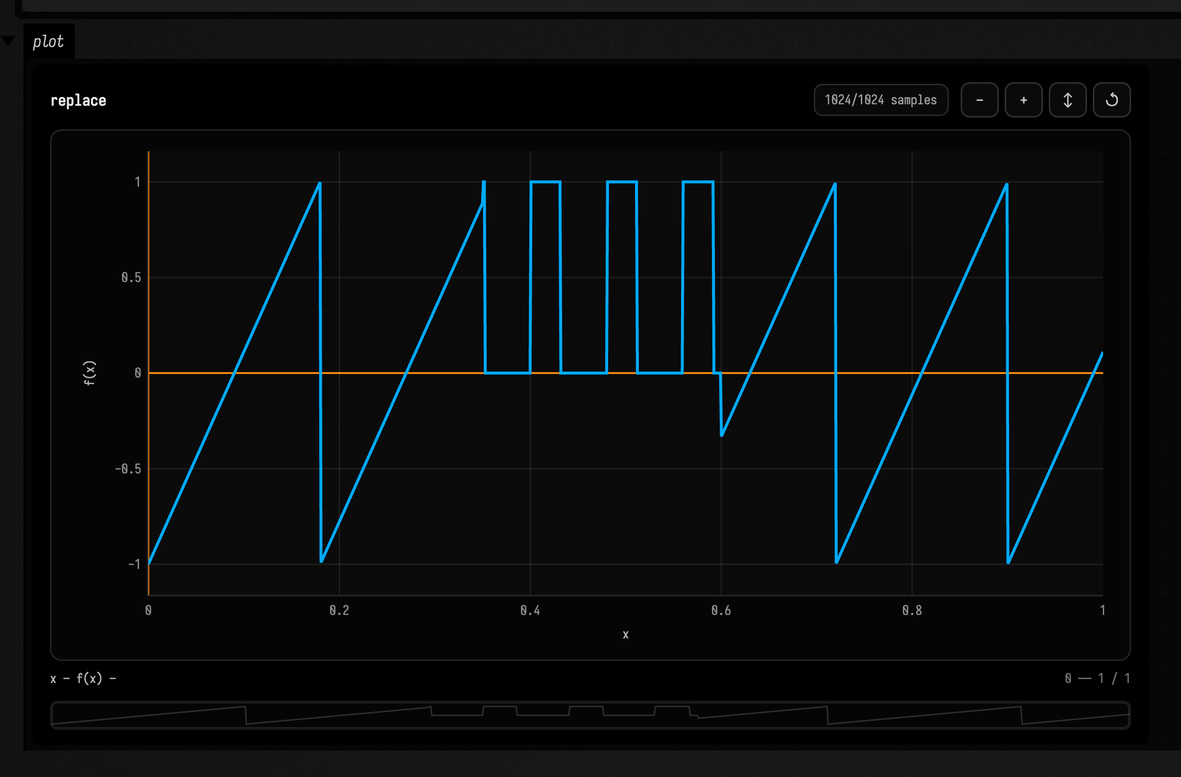
with(Functions) {
    val f = saw(0.18).replace(0.35..0.6, pulseTrain(0.08, duty = 0.4))
    f.plot()
}
window / amplitudeMod / ringMod / warp
Modulation tools multiply, ring, or time-warp one signal by another.
Simple
Multiplies the sine wave by a Hann envelope over the default domain.
val f = sin(2.0).window(hannWindow())Creative
:::static
with(Functions) {
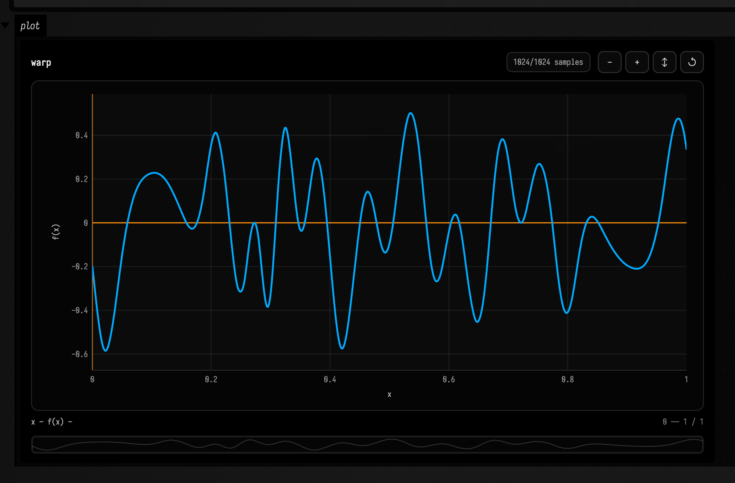
    val f =
        sin(4.0).amplitudeMod(fbm(2, 6.0, 0.7), depth = 0.8).ringMod(cos(9.0), 0.5).warp(valueNoise(2, 5.0, 1.0), 0.05)
    f.plot()
}
quantizeX / sampleHold
X-quantization and sample-hold create stepped time sampling.
Simple
Holds the sine wave constant over 0.05-wide sample steps.
val f = sin(2.0).sampleHold(0.05)Creative
:::static
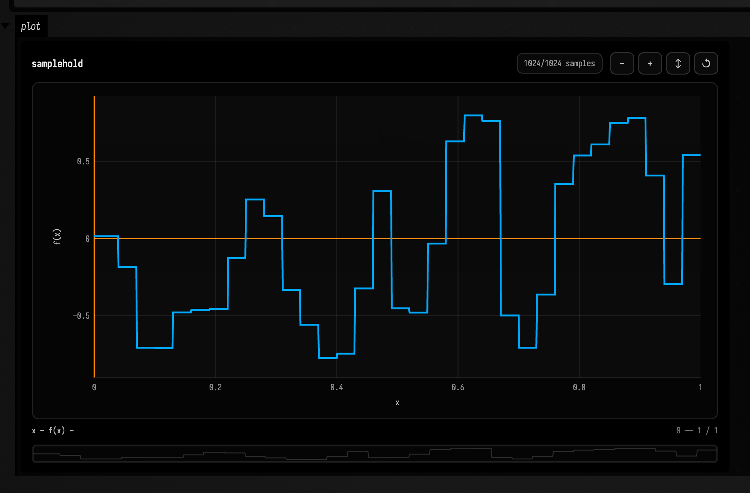
with(Functions) {
    val f = valueNoise(9, 16.0, 0.8).quantizeX(step = ramp(0.02, 0.09)).sampleHold(step = 0.03, offset = 0.01)
    f.plot()
}
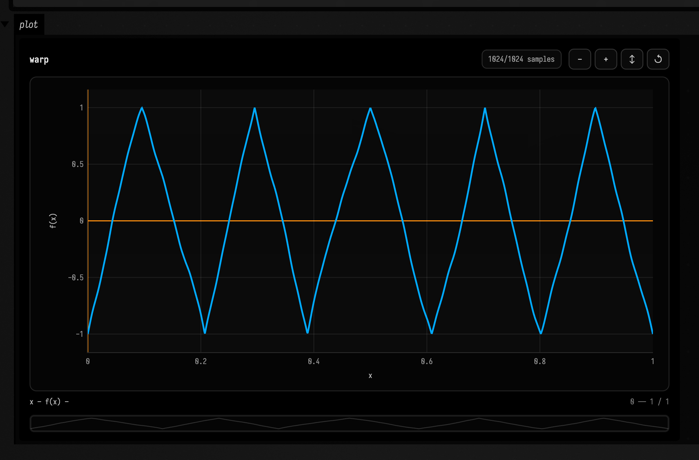
phaseMod / frequencyMod
Phase and frequency modulation are aliases for controlled time warping.
Simple
Modulates the sine wave's phase with a faster sine signal.
val f = sin(2.0).phaseMod(sin(8.0), 0.02)Creative
:::static
with(Functions) {
    val f = triangle(0.2).frequencyMod(fbmPerlin(5, 4.0, 1.0), depth = 0.04)
    f.plot()
}
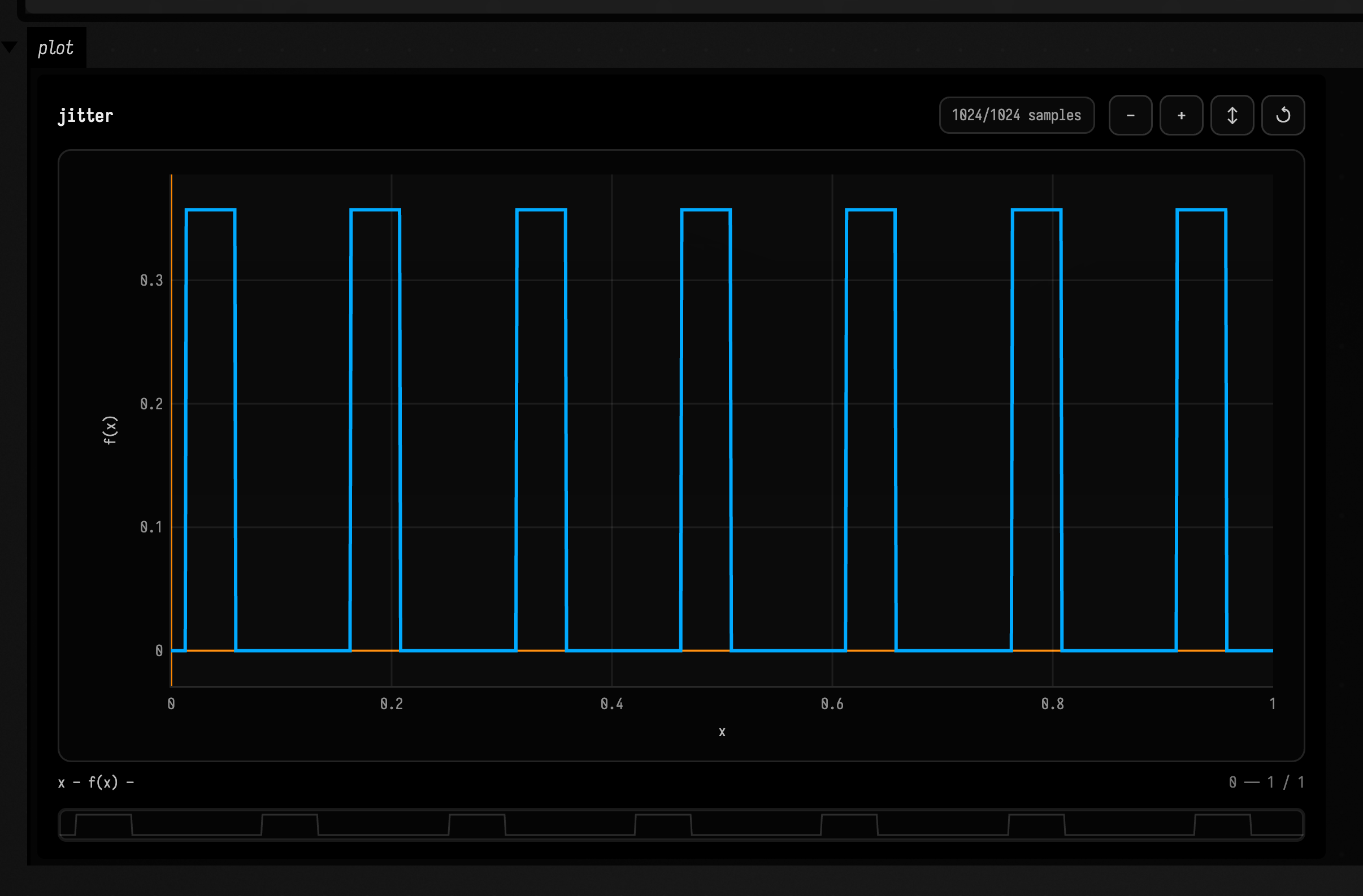
saturate / jitterX
Saturation compresses output values while jitter perturbs sampling positions.
Simple
Pushes the sine through a saturation curve without changing its timing.
val f = sin(2.0).saturate(1.0)Creative
:::static
with(Functions) {
    val f = pulseTrain(0.15, duty = 0.3).jitterX(0.03, seed = 7).saturate(1.8)
    f.plot()
}
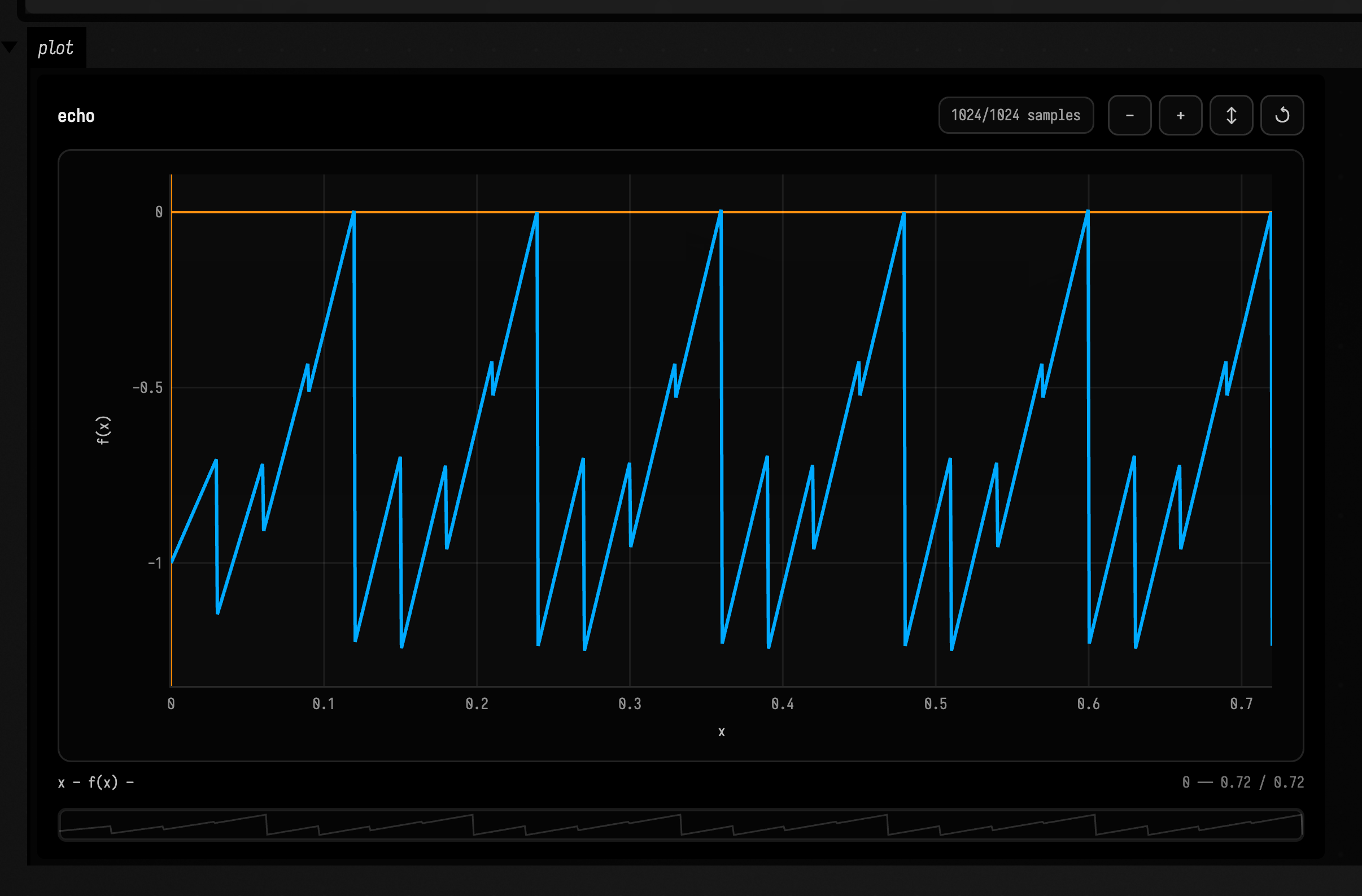
repeat / mirrorRepeat / tile / pad / echo
Repetition tools loop, mirror, bound, extend, and echo a source function.
Simple
Tiles the sine wave into repeated 0.25-wide copies.
val f = sin(2.0).repeat(0.25, 0.0)Creative
:::static
with(Functions) {
    val f = saw(0.2).mirrorRepeat(0.17).tile(6, 0.12).pad(0.05, 0.08, 0.0).echo(0.03, 0.45, repeats = 6)
    f.plot()
}
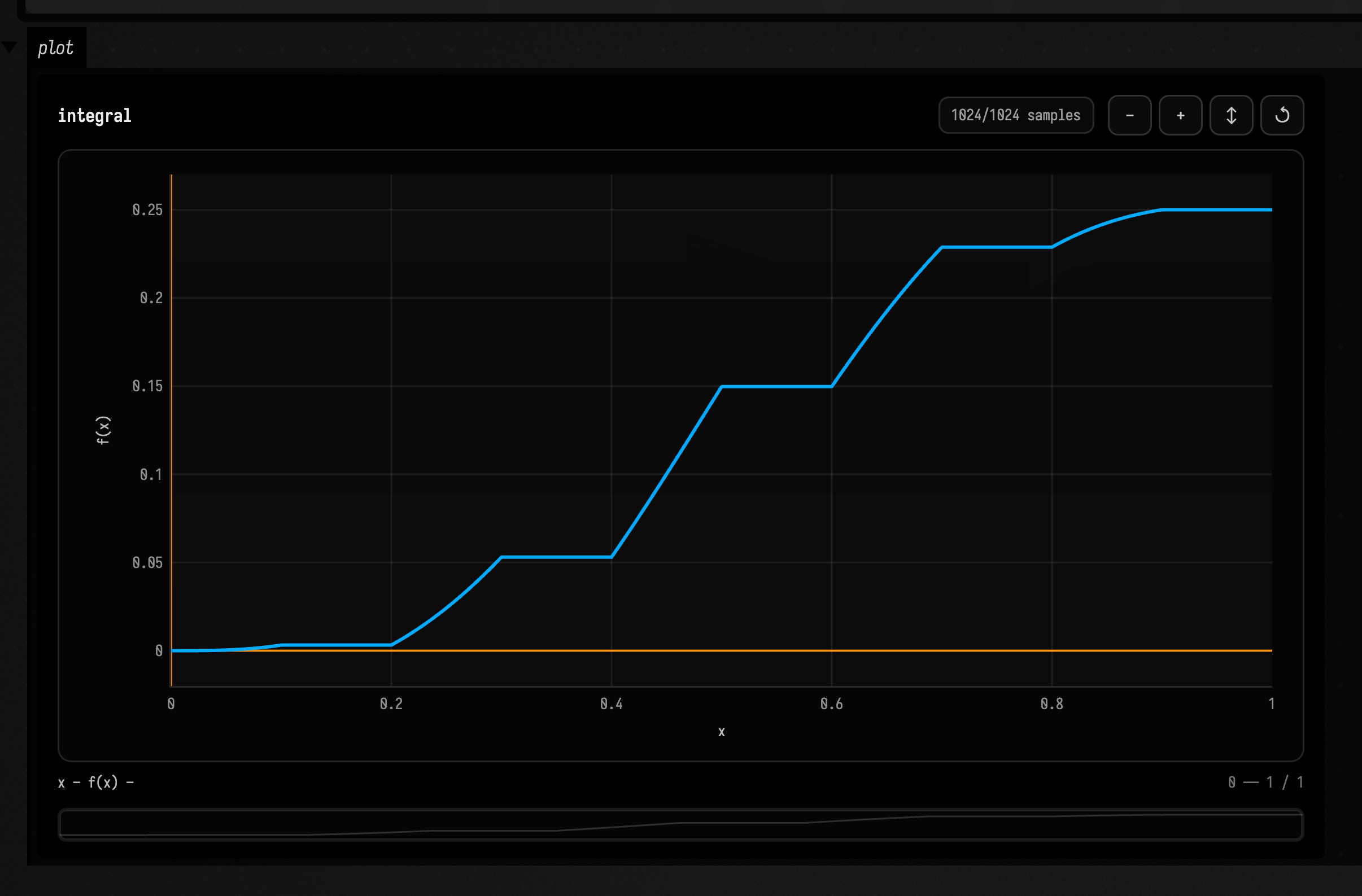
derivative / integral
Calculus helpers estimate slope and accumulated area over a sampled function.
Simple
Estimates the sine wave's slope as a new function.
val slope = sin(2.0).derivative()Creative
:::static
with(Functions) {
    val area = (pulseTrain(0.2) * hannWindow()).integral(step = 1e-3, origin = 0.0)
    area.plot()
}
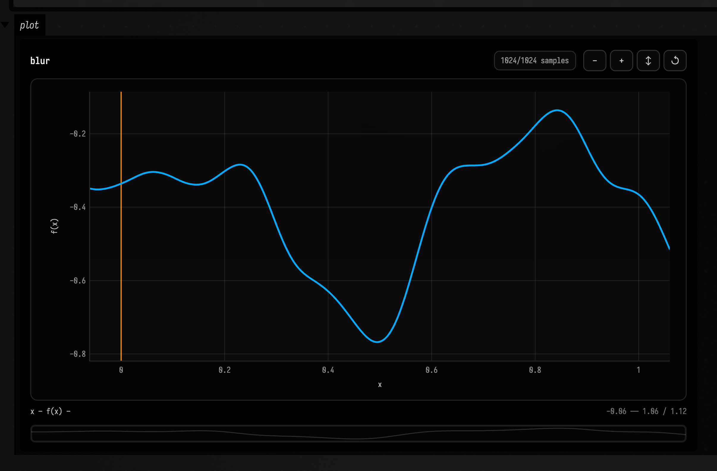
convolve / correlate / movingAverage / blur
Filtering helpers smooth or compare a function with a local kernel.
Simple
Smooths the noise by averaging nearby samples over a short window.
val sm = valueNoise(3, 14.0, 1.0).movingAverage(0.08, samples = 64)Creative
:::static
with(Functions) {
    val f =
        fbm(9, 2.0, 1.0)
            .convolve(
                gaussianWindow(-0.06..0.06, sigma = 0.3),
                samples = 41,
                kernelDomain = -0.06..0.06,
                normalize = true,
            )
            .blur(0.01, samples = 31)
    f.plot()
}
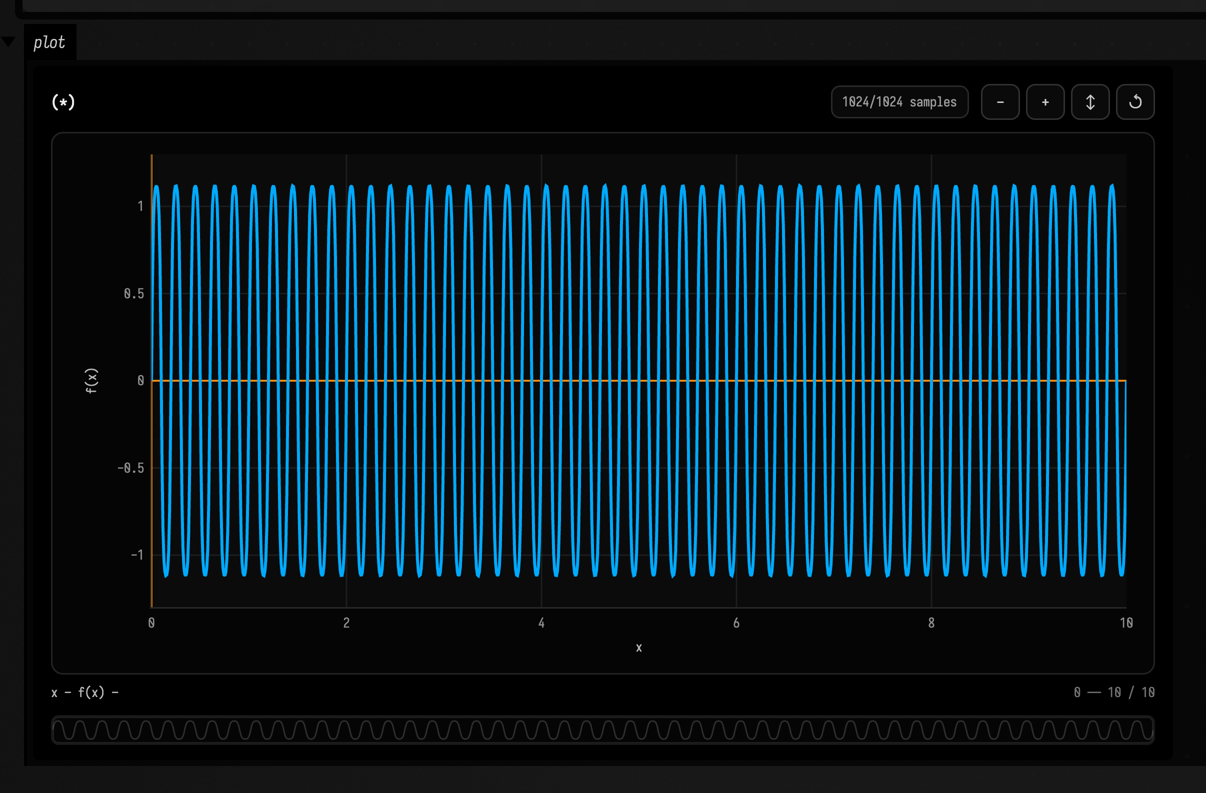
over / stretch / / pipe
over relabels the resulting domain, stretch remaps the old domain into a new one, and / pipes a function through transforms.
Simple
Shows the difference between relabeling a domain and remapping a source into a target interval.
val relabeled = sin(5.0) over (0.0..10.0)
val stretched = sin(5.0) stretch (0.0..10.0)
val piped = sin(5.0) / stretch(0.0..10.0)
Creative
:::static
with(Functions) {
    val f = ((sin(5.0) * 1.4) / delay(0.4) / softClipBy(1.2)) over (0.0..10.0)
    f.plot()
}
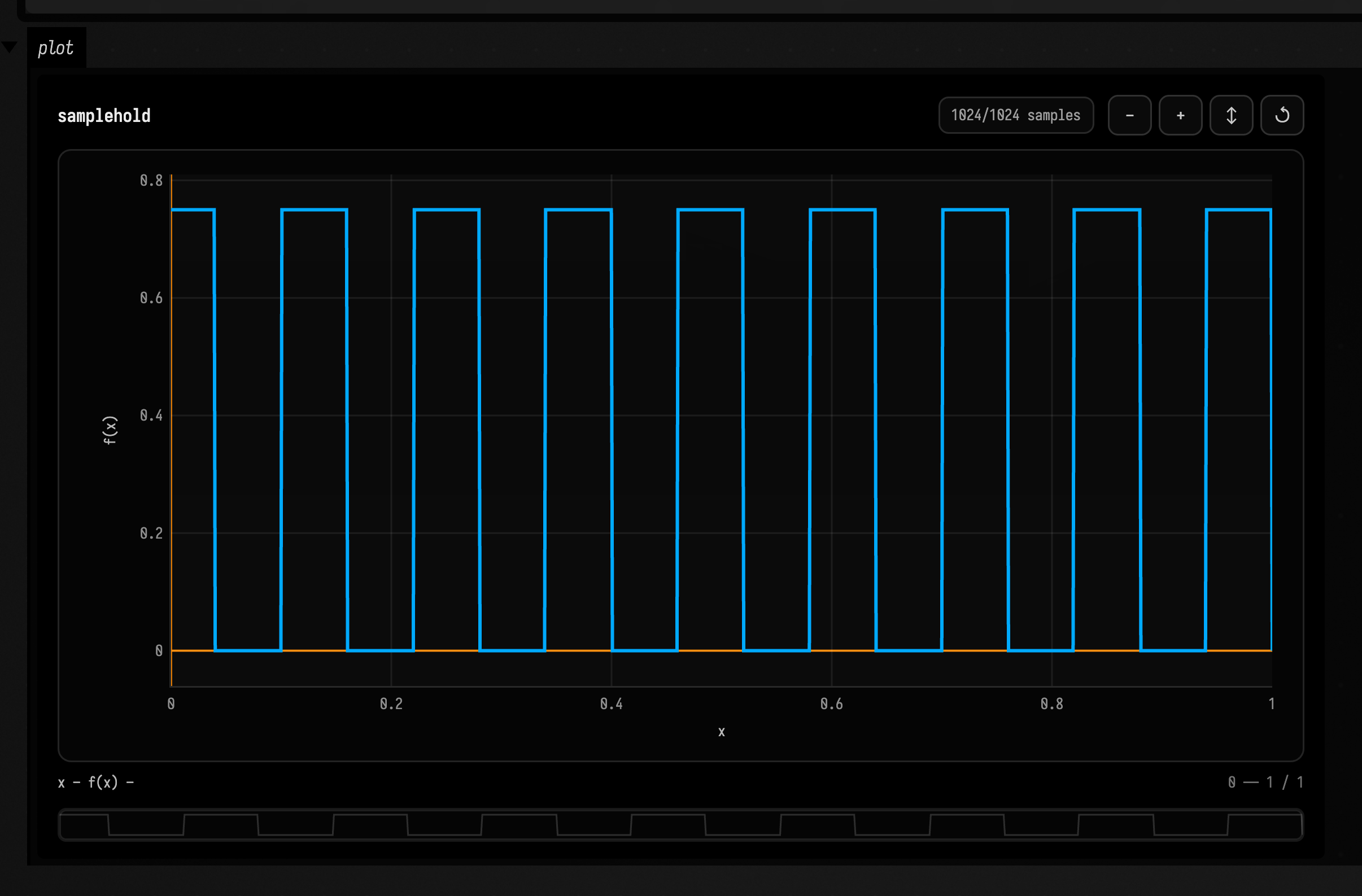
FnTransform
FnTransform packages reusable function edits so they can be chained and piped.
Simple
Pipes the sine wave through a transform that halves its amplitude.
val f = sin(3.0) / gain(0.5)Creative
:::static
with(Functions) {
    val shape = delay(0.1) / gain(0.75) / hold(0.02)
    val f = pulseTrain(0.12) / shape
    f.plot()
}
Arrays, sampling, streams, and output conversion
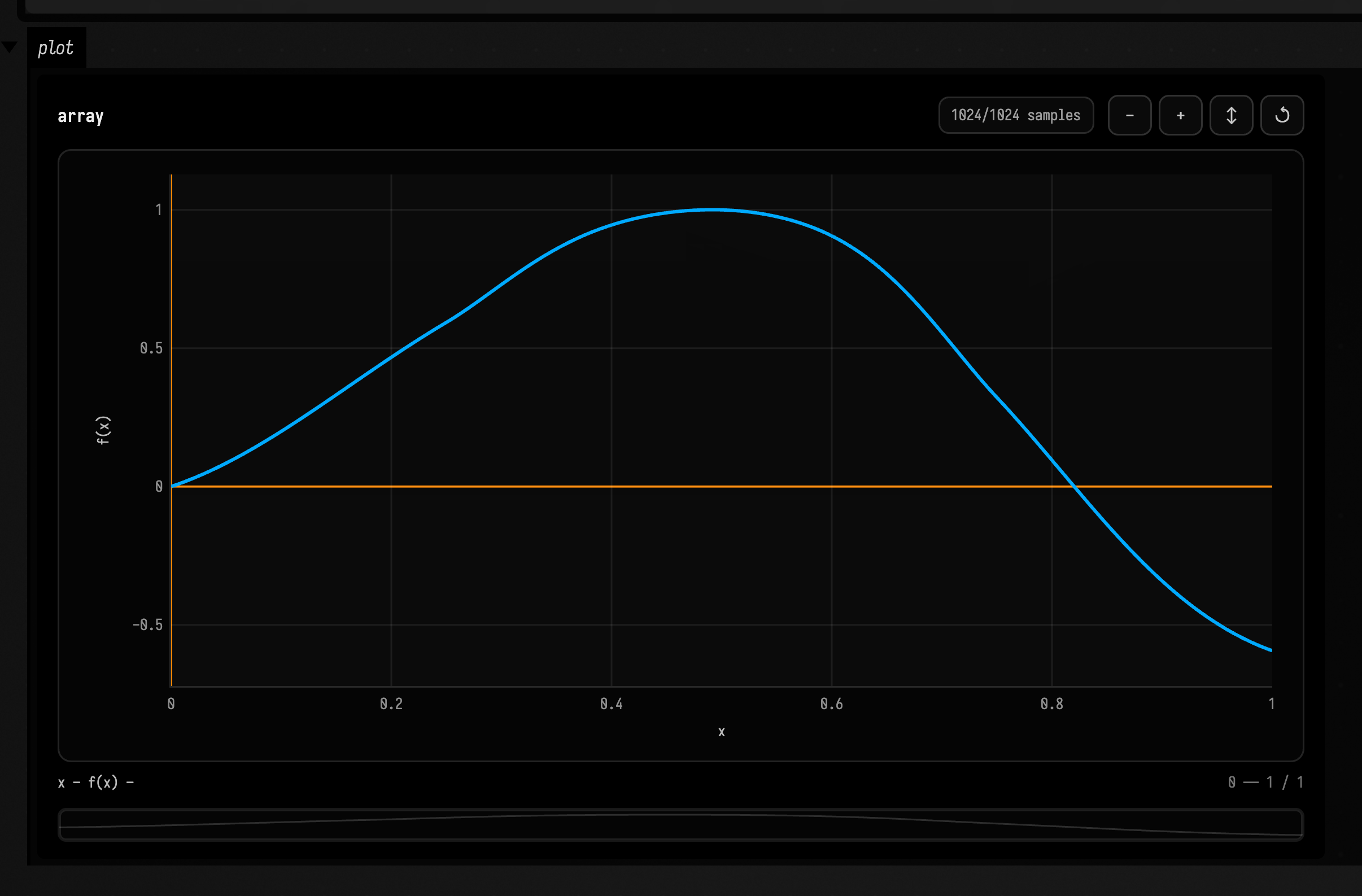
DoubleArray.toFn / List.toFn
Array conversion turns sampled numeric data into an interpolated Fn.
Simple
Interpolates the four array values across 0.0..1.0 as a function.
val f = doubleArrayOf(0.0, 1.0, 0.4, -0.2).toFn(domain = 0.0..1.0)Creative
:::static
with(Functions) {
    val f = [0.0, 0.4, 1.0, 0.2, -0.4].toFn(domain = 0.0..1.0, interpolation = CUBIC).softClip(1.5)
    f.plot()
}
sampleAt / samplesAt
Sampling helpers extract values or weighted sample records from chosen x positions.
Simple
Samples the sine wave at three explicit x positions.
val ys = sin(2.0).sampleAt(doubleArrayOf(0.0, 0.25, 0.5))Creative
:::static
with(Functions) {
    val f = fbmPerlin(8, 2.0, 1.0)
    val pts = f.samplesAt(DoubleArray(32) { it / 31.0 })
    // Screen y grows downward; negate the scale so larger values appear higher.
    val curve = f.toFLine(samples = 600, xScale = 980.0, yScale = -170.0, xOffset = 30.0, yOffset = 220.0)
    curve.color = vec(0.62, 0.95, 1.0, 0.7)
    val markers = pts.map { sample ->
        fline {
            circle(30.0 + sample.x * 980.0, 220.0 - sample.y * 170.0, 4.0)
            color = vec(1.0, 0.75, 0.4, 1.0)
            filled = true
            stroked = false
        }
    }
    lines(curve, *markers.toTypedArray(), channel = "samples", w = 1040.0, h = 440.0, fitToSize = false)
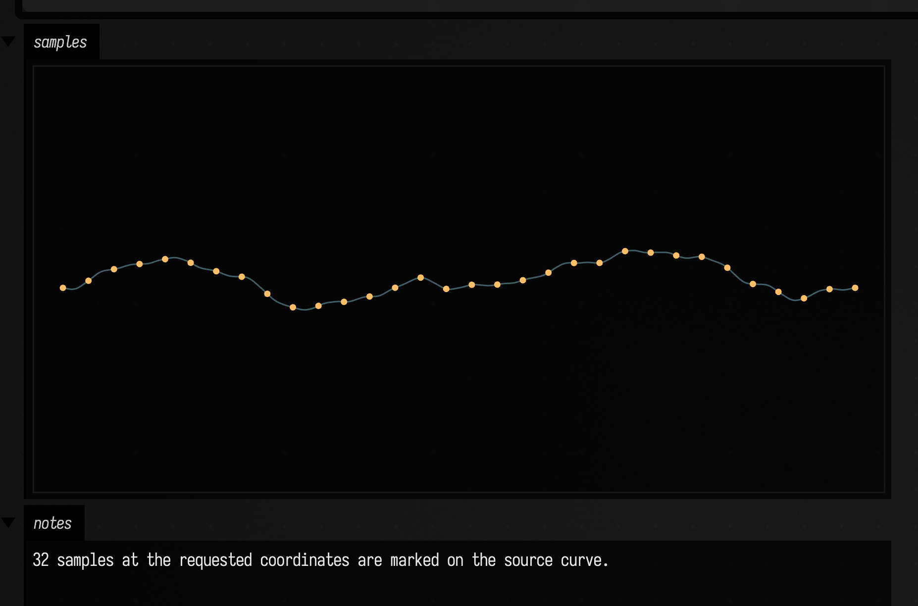
    markdown("notes", "${pts.size} samples at the requested coordinates are marked on the source curve.")
}
toDoubleArray / toVec2List
Array exporters resample an Fn for analysis, drawing, or interop.
Simple
Resamples the sine wave into 128 numeric values.
val ys = sin(3.0).toDoubleArray(128)Creative
:::static
with(Functions) {
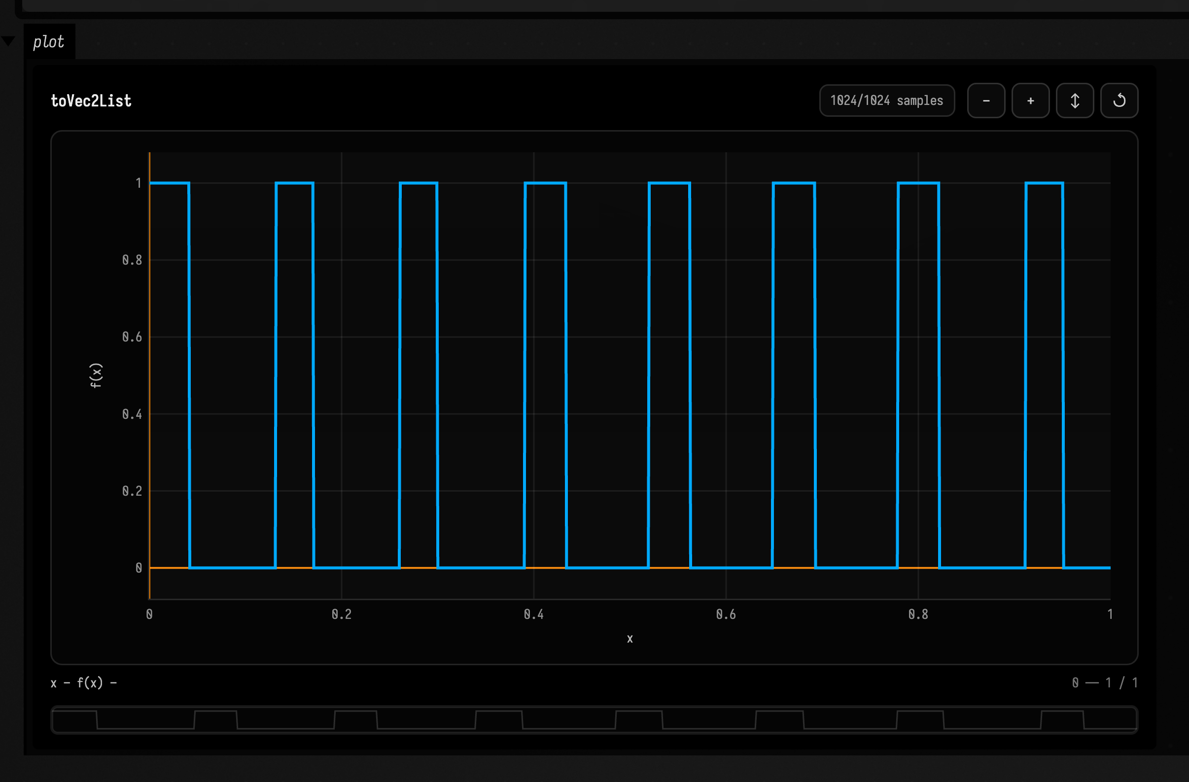
    val pts = pulseTrain(0.13, duty = 0.32).toVec2List(256)
    val f = pts.map { it.y.toDouble() }.toFn(domain = 0.0..1.0, interpolation = NEAREST).withName("toVec2List")
    f.plot()
}
cursor
A cursor walks through a function at a fixed step and remembers its position.
Simple
Creates a reusable cursor that advances through the sine wave in 0.01 steps.
val c0 = sin(2.0).cursor(start = 0.0, step = 0.01)Creative
:::static
with(Functions) {
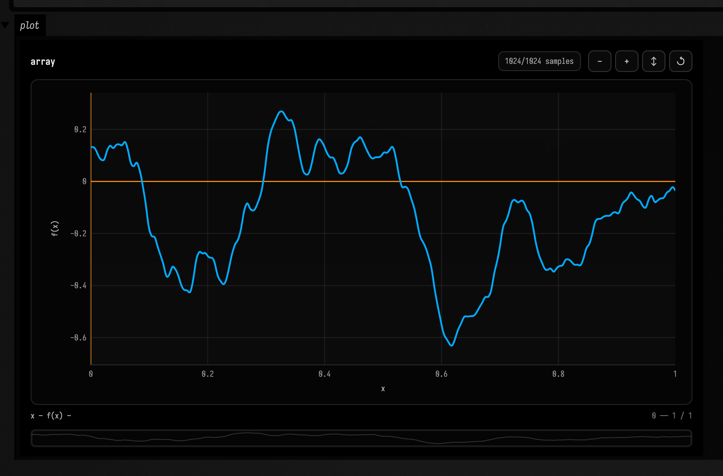
    val scratch = fbm(6, 3.0, 0.8).cursor(0.0, 0.002).next(1024).toFn(0.0..1.0)
    scratch.plot()
}
stream / streamWithX
Streams expose lazy samples, with or without their x coordinate.
Simple
Creates a lazy stream of sine values and collects the first eight samples.
val first = sin(2.0).stream(start = 0.0, step = 0.01).take(8).toList()Creative
:::static
with(Functions) {
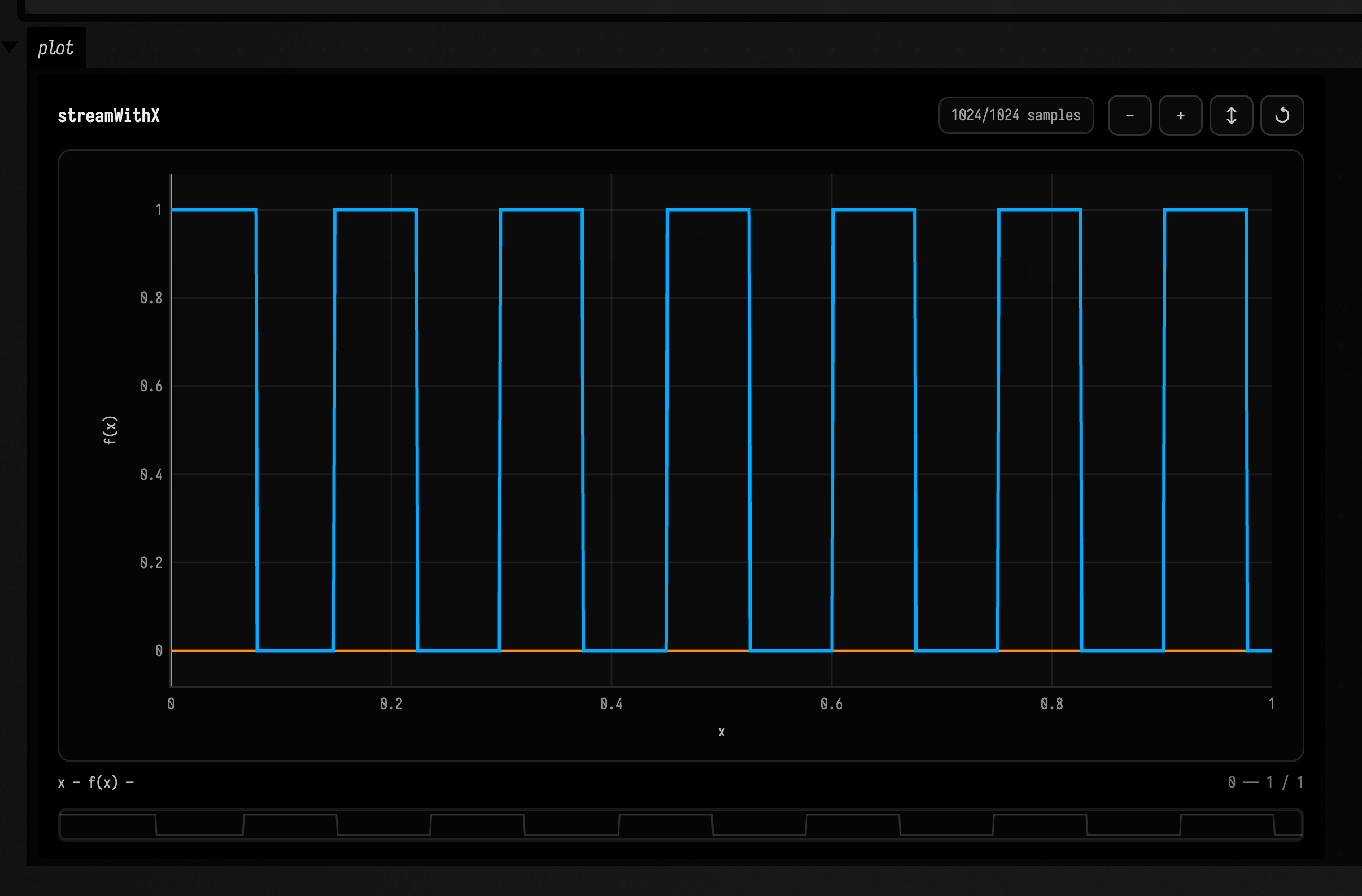
    val pairs = pulseTrain(0.15).streamWithX(0.0, 0.005).take(200).toList()
    val f = pairs.map { it.second }.toFn(domain = 0.0..1.0, interpolation = NEAREST).withName("streamWithX")
    f.plot()
}
toFLine
toFLine turns a sampled function into drawable Field geometry.
Simple
Converts the sine wave into drawable line geometry sampled across its domain.
val line = sin(2.0).toFLine(samples = 600)Creative
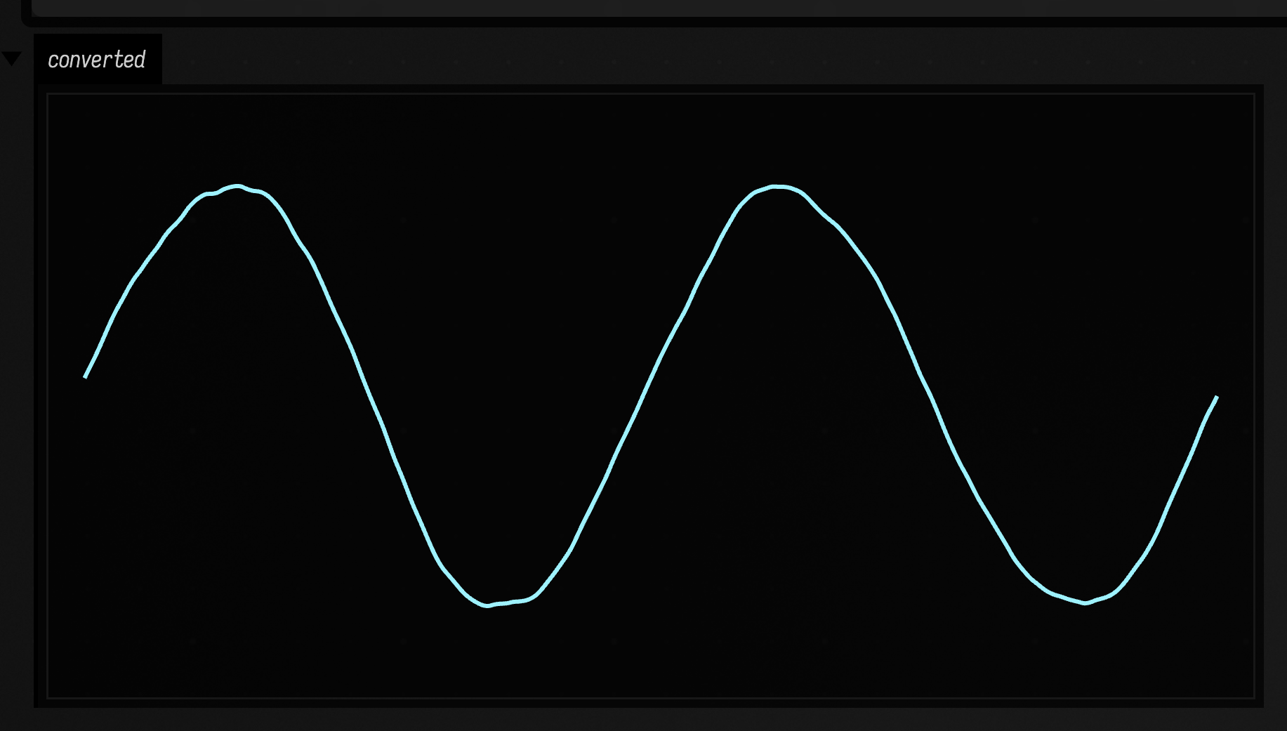
:::static
with(Functions) {
    val f = sin(2.0) + fbm(5, 6.0, 0.2)
    // Screen y grows downward; negate the scale so larger values appear higher.
    val line = f.toFLine(samples = 1400, xScale = 980.0, yScale = -170.0, xOffset = 30.0, yOffset = 220.0)
    line.color = vec(0.62, 0.95, 1.0, 1.0)
    line.thickness = 2.0
    lines(line, channel = "converted", w = 1040.0, h = 440.0, fitToSize = false)
}
Windows, noise, normalization, and sampling sets
hannWindow / hammingWindow / blackmanWindow / gaussianWindow
Window functions create smooth masks for tapering, blending, and weighting.
Simple
Produces a Hann window over the default domain, rising from zero and returning to zero.
val w = hannWindow()Creative
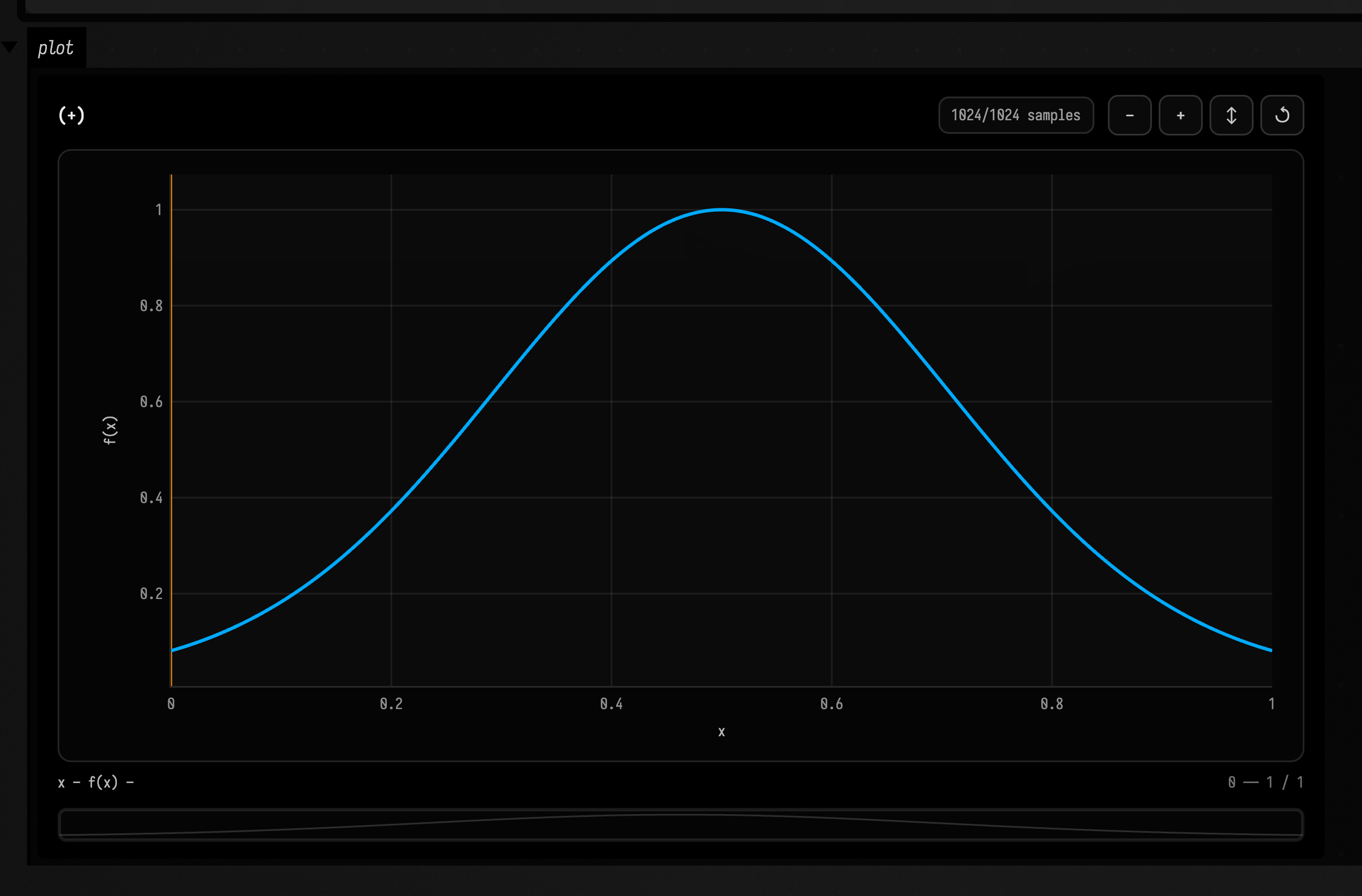
:::static
with(Functions) {
    val w = gaussianWindow(sigma = 0.25).mix(blackmanWindow(), constant(0.4))
    w.plot()
}
whiteNoise / valueNoise / perlinNoise
Noise functions generate stochastic texture with different continuity properties.
Simple
Produces seeded smooth value noise with repeatable random-looking variation.
val n = valueNoise(seed = 1, frequency = 12.0, amplitude = 0.5)Creative
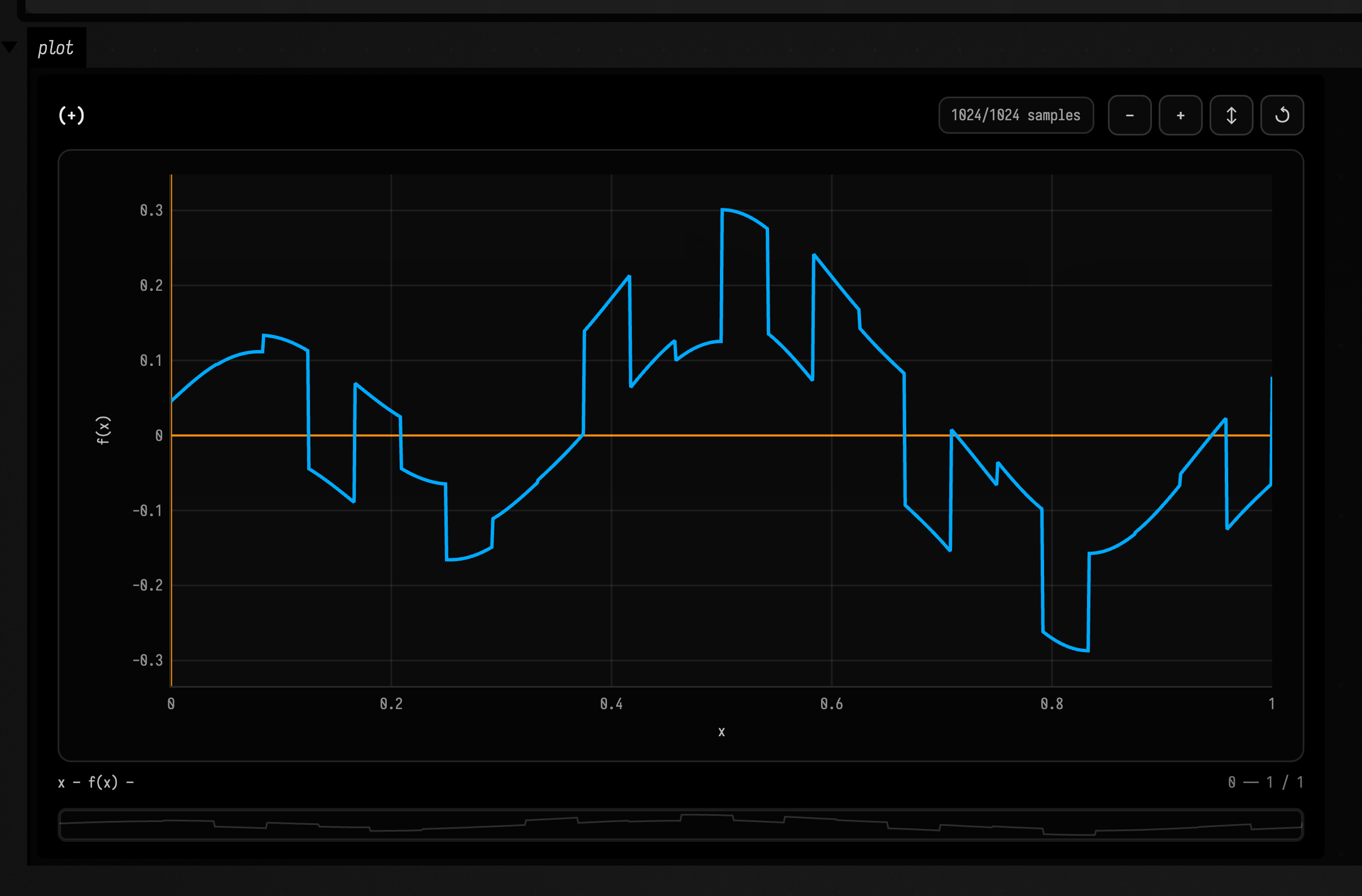
:::static
with(Functions) {
    val n = whiteNoise(4, 24.0, 0.3).mix(perlinNoise(5, 3.0, 0.7), constant(0.65))
    n.plot()
}
fbm / fbmPerlin / randomWalk
Fractal and walk generators layer randomness into rougher, multi-scale signals.
Simple
Produces layered fractal noise by summing several octaves.
val n = fbm(seed = 2, frequency = 2.0, amplitude = 1.0, octaves = 5)Creative
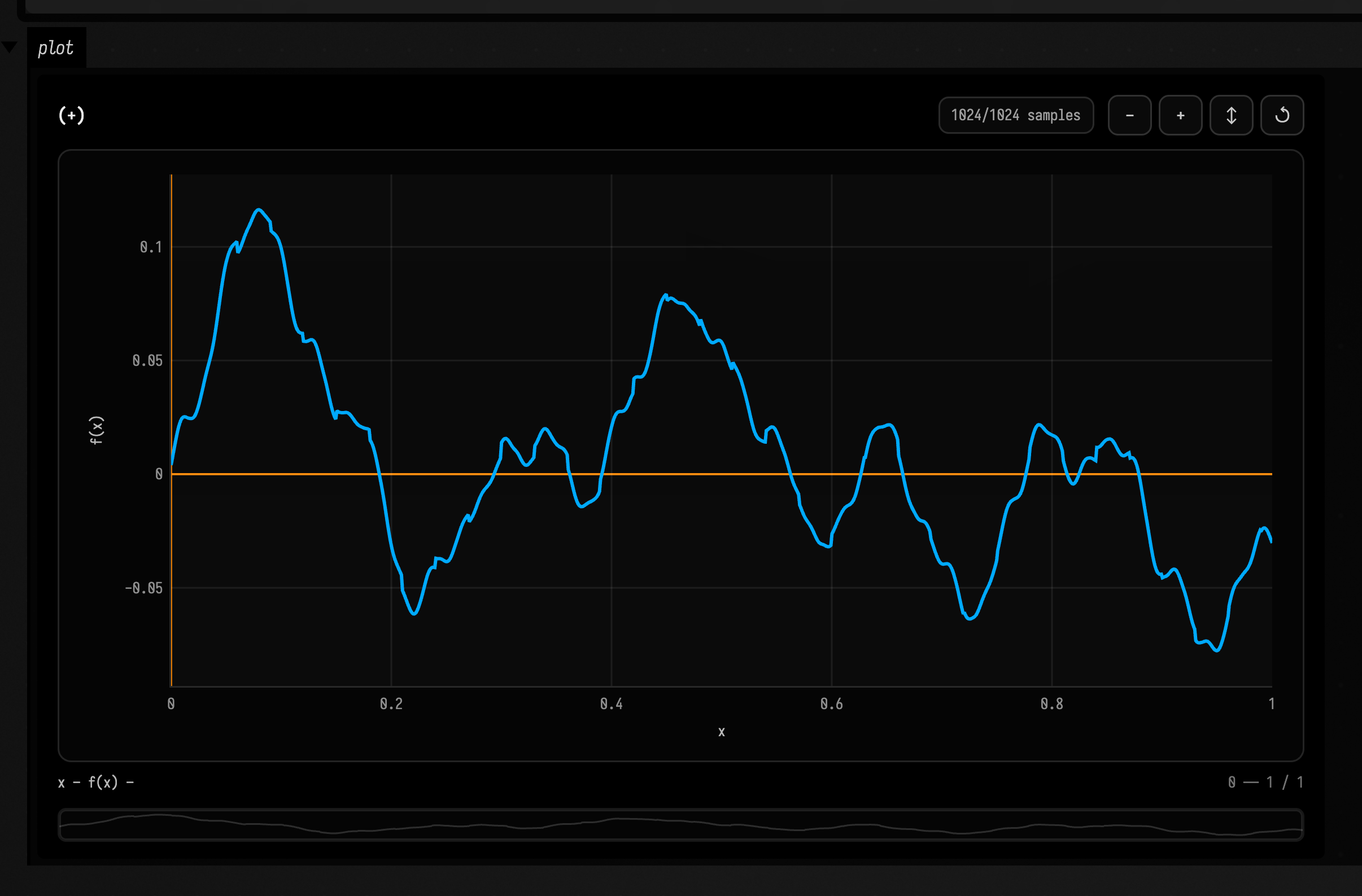
:::static
with(Functions) {
    val n = fbmPerlin(4, 1.8, 1.0, octaves = 6).mix(randomWalk(8, step = 0.03, amplitude = 0.02), constant(0.3))
    n.plot()
}
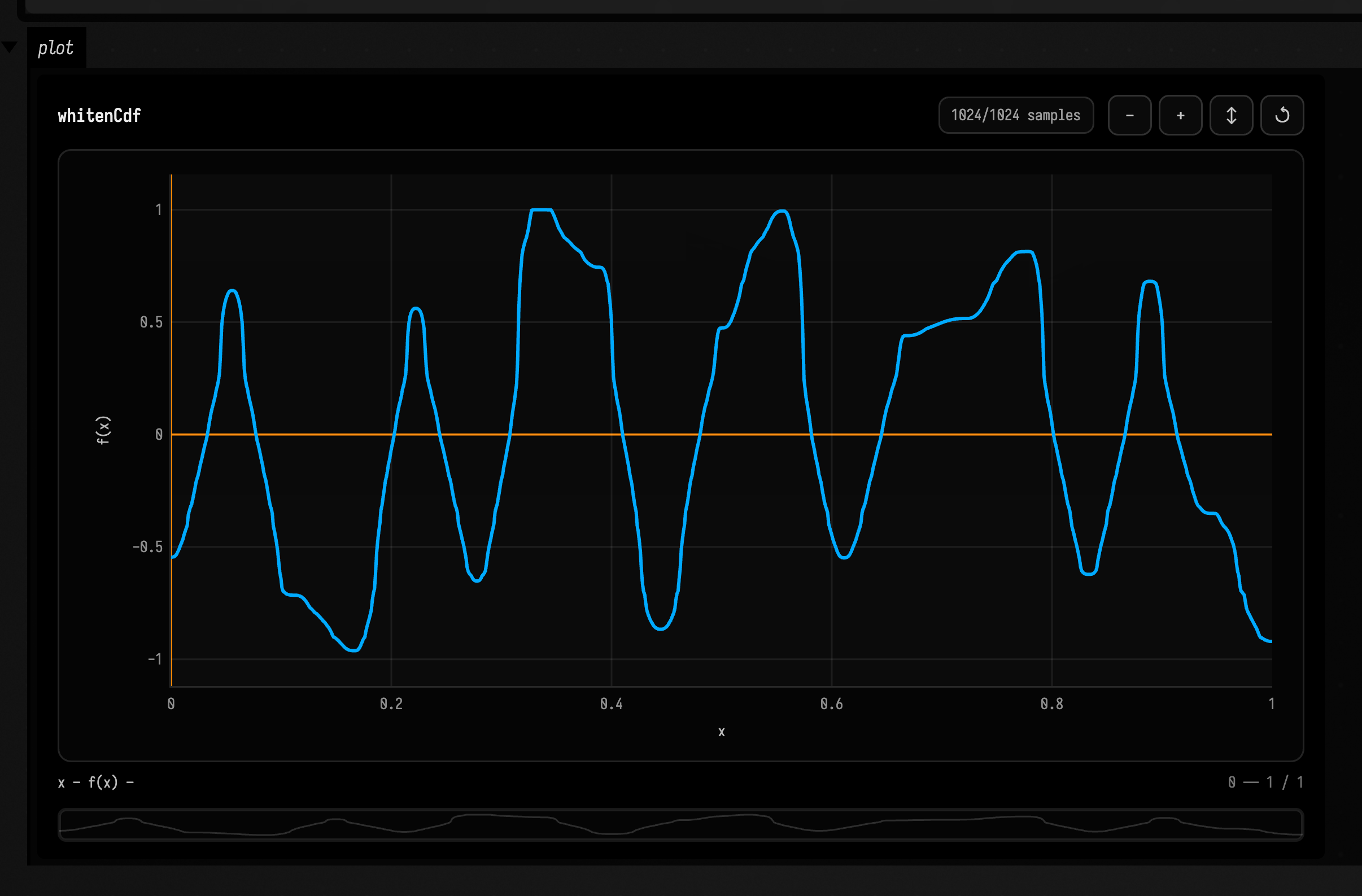
autoScale / zNormalize / whitenCdf
Normalization helpers reshape the distribution of a sampled function.
Simple
Rescales the sampled noise so its values fit a normalized range.
val f = fbm(4, 2.0, 1.0).autoScale()Creative
:::static
with(Functions) {
    val f = valueNoise(12, 18.0, 1.0).zNormalize().whitenCdf(bins = 128, targetMin = -1.0, targetMax = 1.0)
    f.plot()
}
sampleUniform / sampleJittered / sampleRandom
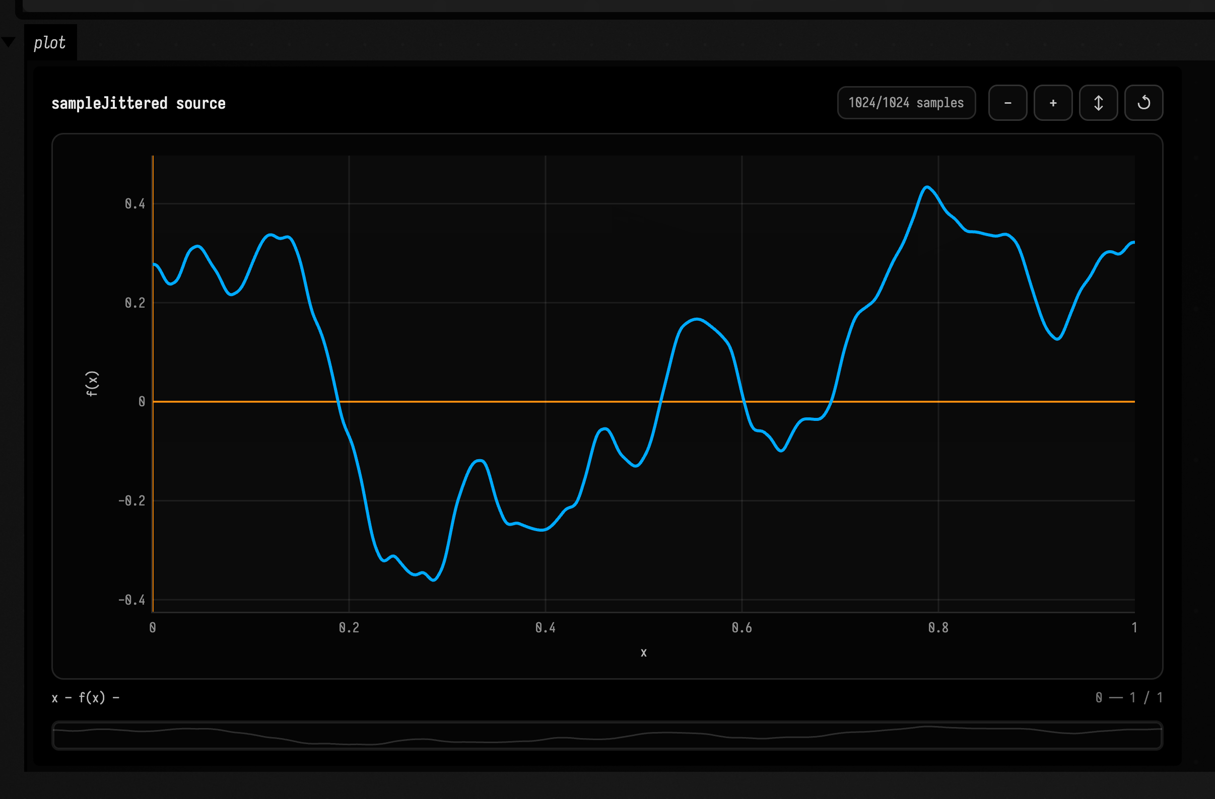
Sampling-set helpers choose x positions uniformly, randomly, or with jitter.
Simple
Returns 32 evenly spaced samples from the sine wave.
val s = sin(2.0).sampleUniform(32)Creative
:::static
with(Functions) {
    val f = fbm(2, 3.0, 1.0)
    val s = f.sampleJittered(128, jitter = 0.4, seed = 9)
    f.withName("sampleJittered source").plot()
}
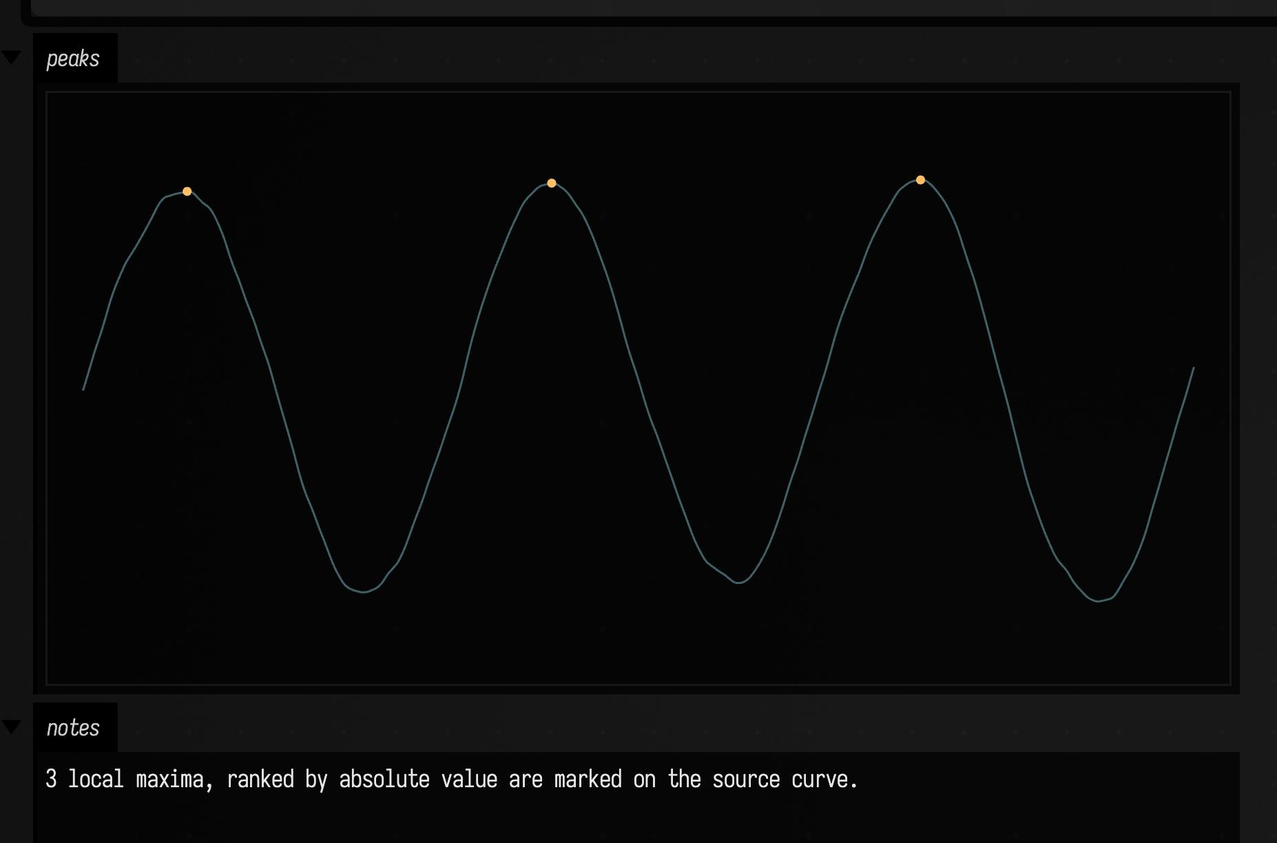
sampleByDensity / sampleZeroCrossings / samplePeaks
Feature samplers find points by density, zero crossings, or prominent peaks.
Simple
Finds x positions where the sine wave crosses zero.
val zc = sin(6.0).sampleZeroCrossings()Creative
:::static
with(Functions) {
    val source = sin(3.0) + fbm(1, 7.0, 0.25)
    val peaks = source.samplePeaks(20)
    // Screen y grows downward; negate the scale so larger values appear higher.
    val curve = source.toFLine(samples = 600, xScale = 980.0, yScale = -170.0, xOffset = 30.0, yOffset = 220.0)
    curve.color = vec(0.62, 0.95, 1.0, 0.7)
    val markers = peaks.map { sample ->
        fline {
            circle(30.0 + sample.x * 980.0, 220.0 - sample.y * 170.0, 4.0)
            color = vec(1.0, 0.75, 0.4, 1.0)
            filled = true
            stroked = false
        }
    }
    lines(curve, *markers.toTypedArray(), channel = "peaks", w = 1040.0, h = 440.0, fitToSize = false)
    markdown("notes", "${peaks.size} local maxima, ranked by absolute value are marked on the source curve.")
}
Piecewise, interpolation, RBF, and resampling
points
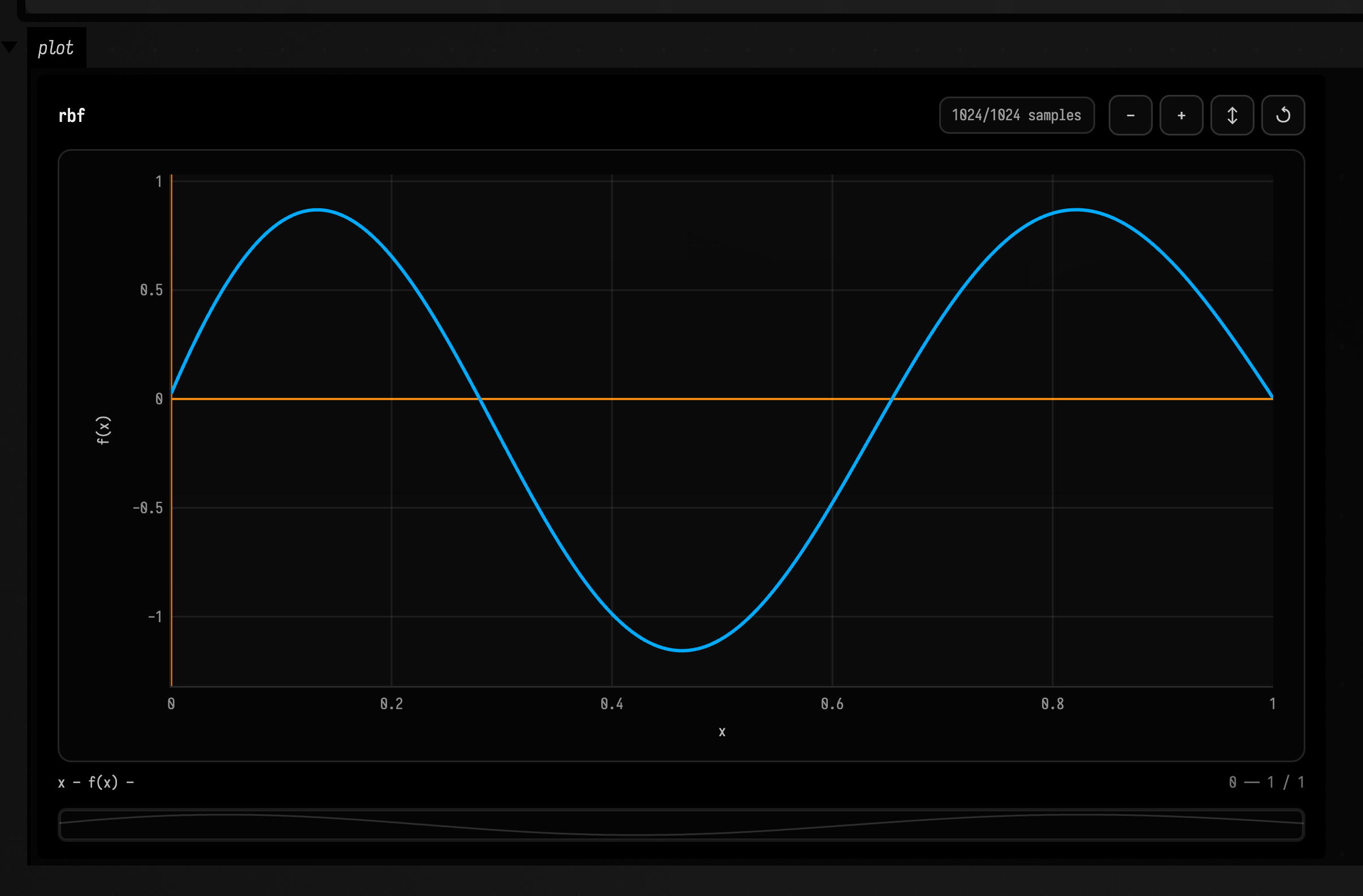
points creates weighted sample records for fitting and interpolation helpers.
Simple
Makes reusable point data from explicit coordinate pairs.
val pts = points(0.0 to 0.0, 0.4 to 1.0, 1.0 to 0.2)Creative
:::static
with(Functions) {
    val pts = points(0.0 to 0.0, 0.12 to 0.9, 0.32 to -0.4, 0.75 to 0.7, 1.0 to 0.0)
    val f = rbf(pts, kernel = RbfKernels.gaussian(2.4), smoothing = 1e-3) over (0.0..1.0)
    f.plot()
}
piecewise
piecewise chooses different source functions over explicit subranges.
Simple
Chooses different source functions over the two specified intervals.
val f = piecewise(zero(), 0.0..0.5 to one(), 0.5..1.0 to zero())Creative
:::static
with(Functions) {
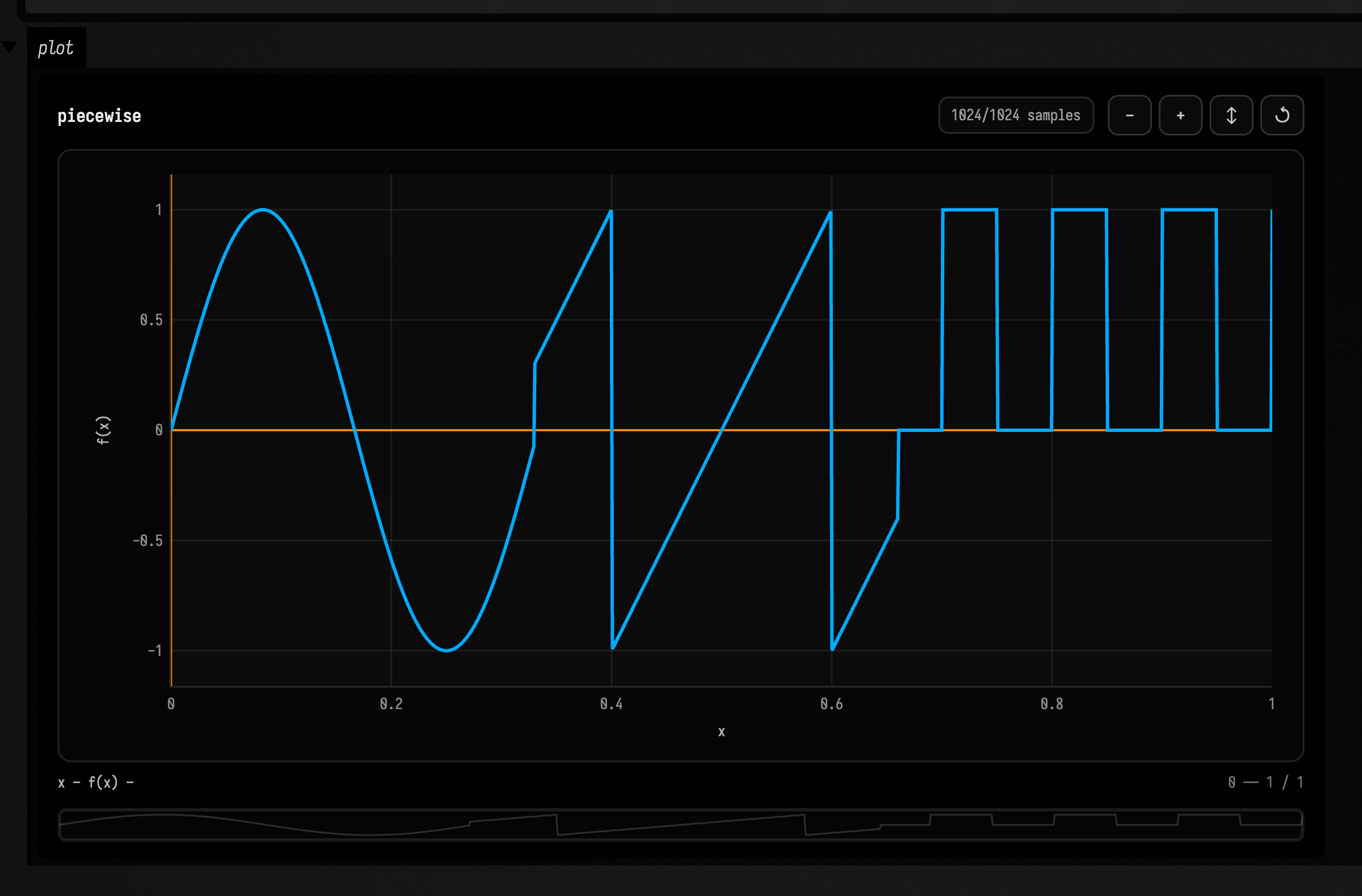
    val f = piecewise(
        default = valueNoise(3, 8.0, 0.1),
        0.0..0.33 to sin(3.0),
        0.33..0.66 to saw(0.2),
        0.66..1.0 to pulseTrain(0.1),
    )
    f.plot()
}
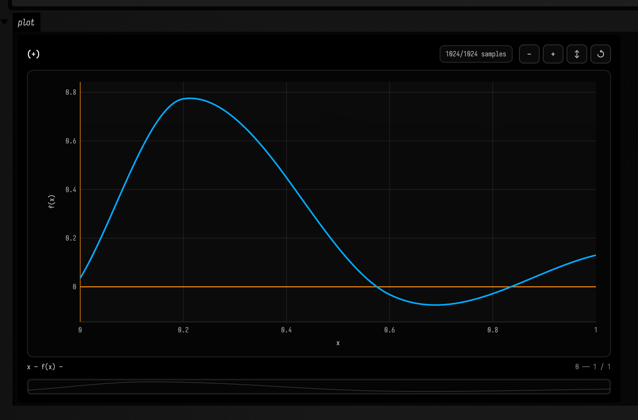
piecewiseLinear / catmullRomSpline / monotoneCubic
Spline constructors turn keyframes into continuous curves with different interpolation behavior.
Simple
Linearly interpolates between two keyframes.
val f = piecewiseLinear([Keyframe(0.0, 0.0, "linear"), Keyframe(1.0, 1.0, "linear")])Creative
:::static
with(Functions) {
    val f =
        catmullRomSpline(
                [
                    Keyframe(0.0, 0.0, "linear"),
                    Keyframe(0.2, 0.9, "linear"),
                    Keyframe(0.6, -0.4, "linear"),
                    Keyframe(1.0, 0.2, "linear"),
                ],
                alpha = 0.5,
            )
            .mix(
                monotoneCubic(
                    [Keyframe(0.0, 0.1, "linear"), Keyframe(0.4, 0.8, "linear"), Keyframe(1.0, 0.0, "linear")],
                ),
                constant(0.35),
            )
    f.plot()
}
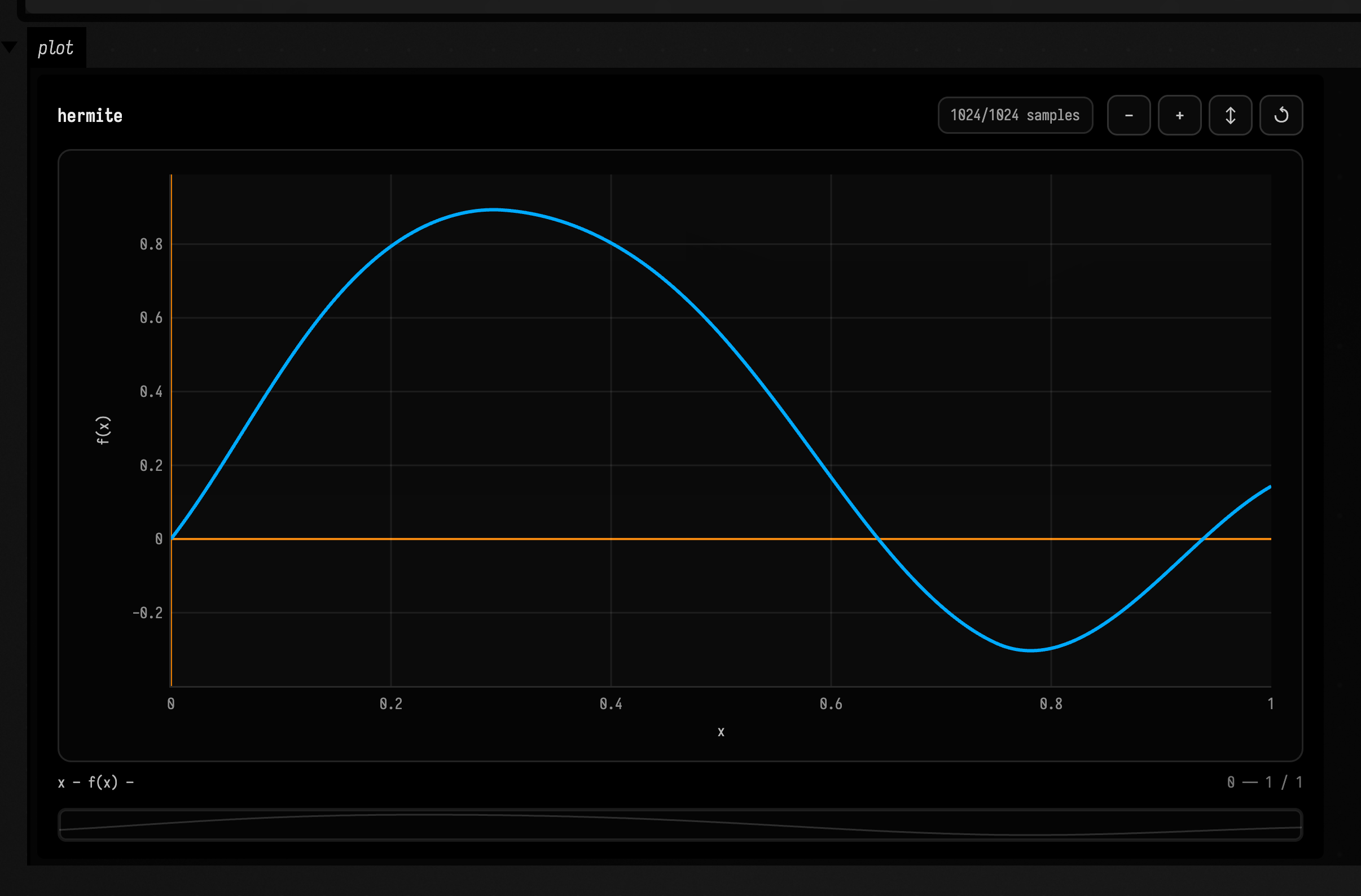
hermiteFromHandles / bSplineQuadratic
Handle and B-spline helpers make smoother keyframe-derived curves.
Simple
Builds a smooth quadratic B-spline through the keyframe values.
val f = bSplineQuadratic([Keyframe(0.0, 0.0, "linear"), Keyframe(0.4, 1.0, "linear"), Keyframe(1.0, 0.2, "linear")])Creative
:::static
with(Functions) {
    val f =
        hermiteFromHandles(
                [
                    Keyframe(0.0, 0.0, "linear"),
                    Keyframe(0.3, 0.8, "linear"),
                    Keyframe(0.75, -0.2, "linear"),
                    Keyframe(1.0, 0.1, "linear"),
                ],
            )
            .softClip(constant(1.2))
    f.plot()
}
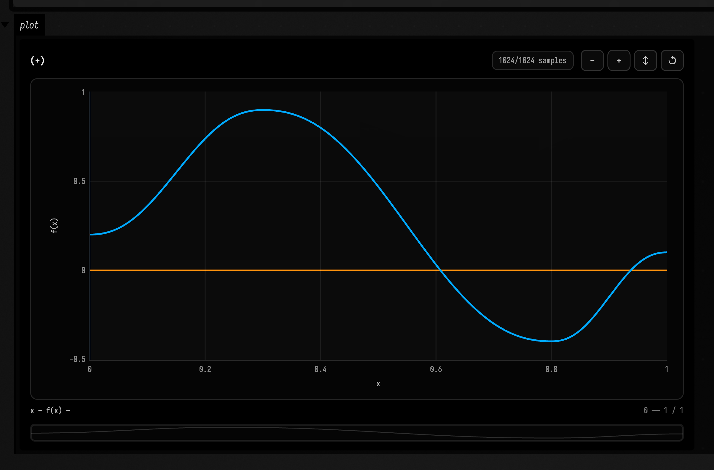
stepHold / nearestValue / cosineInterp / smoothStepInterp / smootherStepInterp
Discrete and eased interpolators choose how keyframes are held or blended.
Simple
Holds each keyframe value until the next keyframe is reached.
val f = stepHold([Keyframe(0.0, 0.0, "linear"), Keyframe(0.5, 1.0, "linear"), Keyframe(1.0, 0.5, "linear")])Creative
:::static
with(Functions) {
    val f =
        cosineInterp(
                [
                    Keyframe(0.0, 0.2, "linear"),
                    Keyframe(0.3, 0.9, "linear"),
                    Keyframe(0.8, -0.4, "linear"),
                    Keyframe(1.0, 0.1, "linear"),
                ],
            )
            .mix(
                smootherStepInterp(
                    [
                        Keyframe(0.0, 0.2, "linear"),
                        Keyframe(0.3, 0.9, "linear"),
                        Keyframe(0.8, -0.4, "linear"),
                        Keyframe(1.0, 0.1, "linear"),
                    ],
                ),
                constant(0.5),
            )
    f.plot()
}
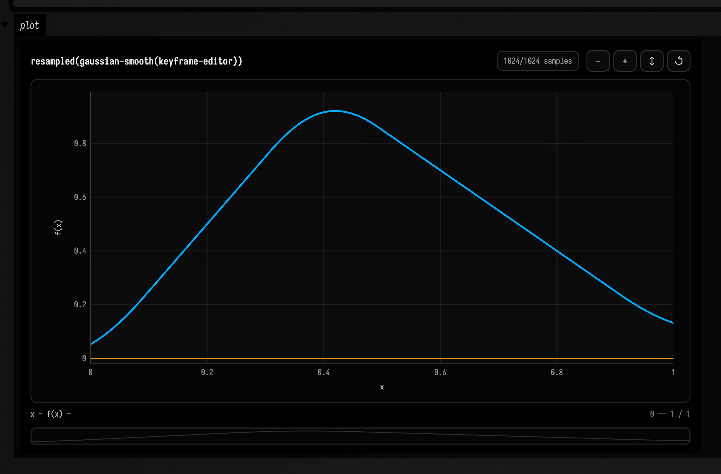
gaussianSmooth / differentiate / fromKeyframeEditor / resample
Curve utilities smooth, differentiate, import, and resample keyframed functions.
Simple
Approximates the derivative of the sine wave.
val f = differentiate(sin(2.0))Creative
:::static
with(Functions) {
    val f =
        gaussianSmooth(
                fromKeyframeEditor(
                    [Keyframe(0.0, 0.0, "linear"), Keyframe(0.4, 1.0, "bezier"), Keyframe(1.0, 0.1, "linear")],
                ),
                sigma = 0.03,
                taps = 41,
            )
            .let { resample(it, sampleCount = 512, interpolation = CUBIC) }
    f.plot()
}
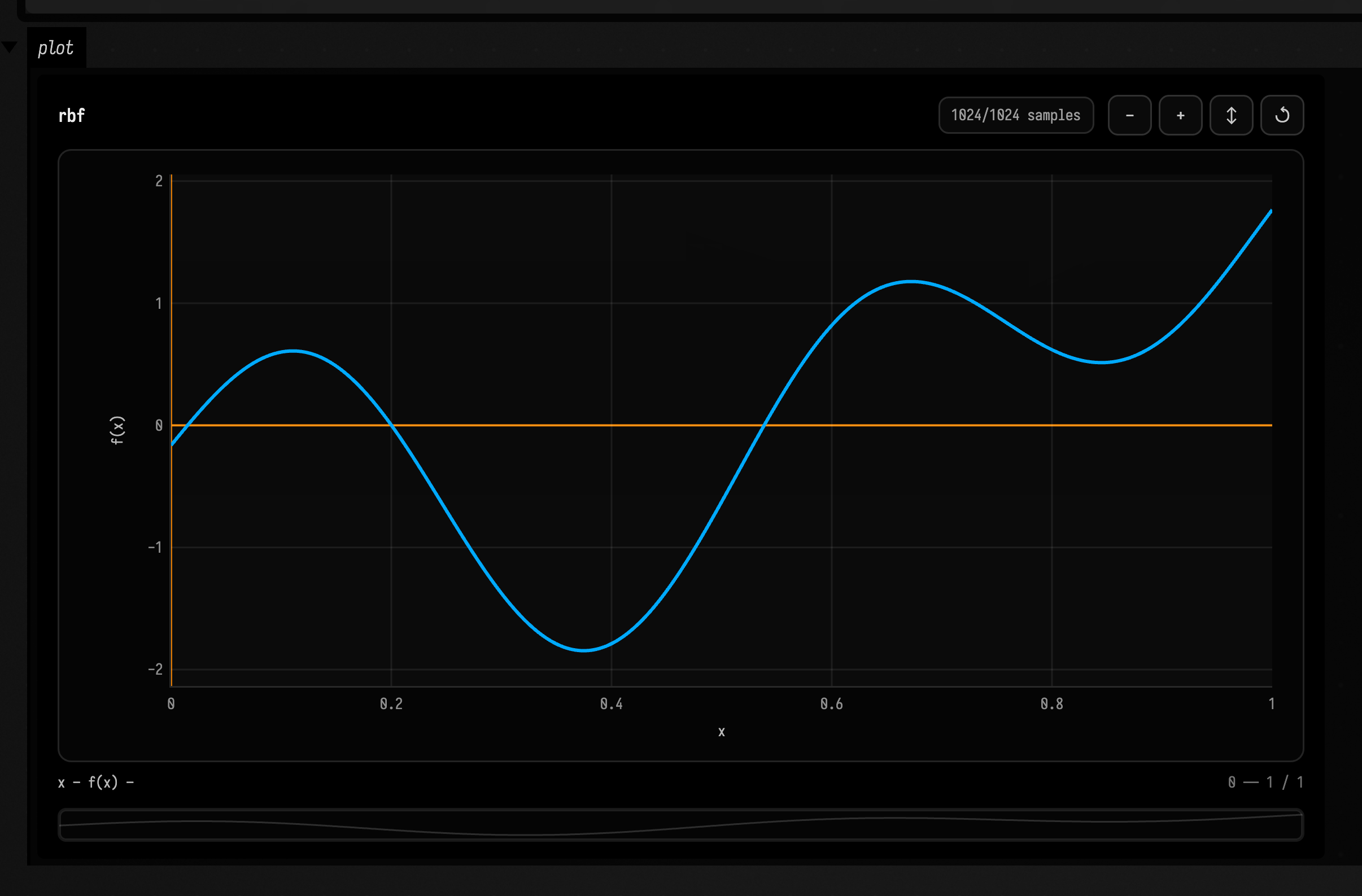
rbf / rbfQuadratic / rbfCubic / rbfThinPlate and Fn.* variants
RBF helpers fit smooth curves through scattered samples, optionally blended with a base function.
Simple
Interpolates the points with a thin-plate radial basis function.
val f = rbfThinPlate(points(0.0 to 0.0, 0.4 to 1.0, 1.0 to 0.2))Creative
:::static
with(Functions) {
    val f =
        sin(2.0).rbf(points(0.1 to 0.6, 0.52 to -0.3, 0.9 to 0.7), kernel = RbfKernels.gaussian(2.5), smoothing = 1e-4)
    f.plot()
}
rbfField: radial basis functions in two dimensions
rbfField fits a surface through values scattered over a plane, the 2D counterpart of rbf, with the
same RbfKernels. Give it a list of point to value pairs and call the result like a function, at a
Vec2 or at x, y. It is top level rather than inside Functions, because what it returns is a
surface, not a curve.
Simple
Fits a surface through four samples and evaluates it between them.
val field = rbfField([vec(0, 0) to 0.0, vec(1, 0) to 1.0, vec(0, 1) to 1.0, vec(1, 1) to 0.0])
val middle = field(0.5, 0.5)
Creative
Sixty samples of a function over a 2 × 2 square, the surface fitted through them, and ten times the difference between the two:
// 60 samples of a function scattered over a 2 × 2 square, and the surface rbfField fits through them
val rnd = java.util.Random(3)
fun f(x: Double, y: Double) = sin(3 * x) * cos(2 * y) + 0.3 * x
val samples = List(60) {
    val p = vec(rnd.nextDouble() * 2, rnd.nextDouble() * 2)
    p to f(p.x.toDouble(), p.y.toDouble())
}
val field = rbfField(samples)

// how well each sample is predicted by the other 59: the way to compare kernels
println("leave-one-out RMSE, thin plate: " + field.leaveOneOutRmse().f4)
println(
    "leave-one-out RMSE, gaussian(2): " + rbfField(samples, RbfKernels.gaussian(2.0)).leaveOneOutRmse().f4,
)

fun image(g: (Double, Double) -> Double) = Img(
    200,
    200,
    1,
    FloatArray(200 * 200) {
        g((it % 200) / 100.0, (it / 200) / 100.0).toFloat()
    },
)
showImg(
    montage(
        [
            "the function" to image(::f).colormap("coolwarm", -1.4f, 1.4f),
            "the fit" to image { x, y -> field(x, y) }.colormap("coolwarm", -1.4f, 1.4f),
            "error x 10" to image { x, y -> 10 * (field(x, y) - f(x, y)) }.colormap("coolwarm", -1.4f, 1.4f),
        ],
        columns = 3,
        cellSide = 260,
    ),
)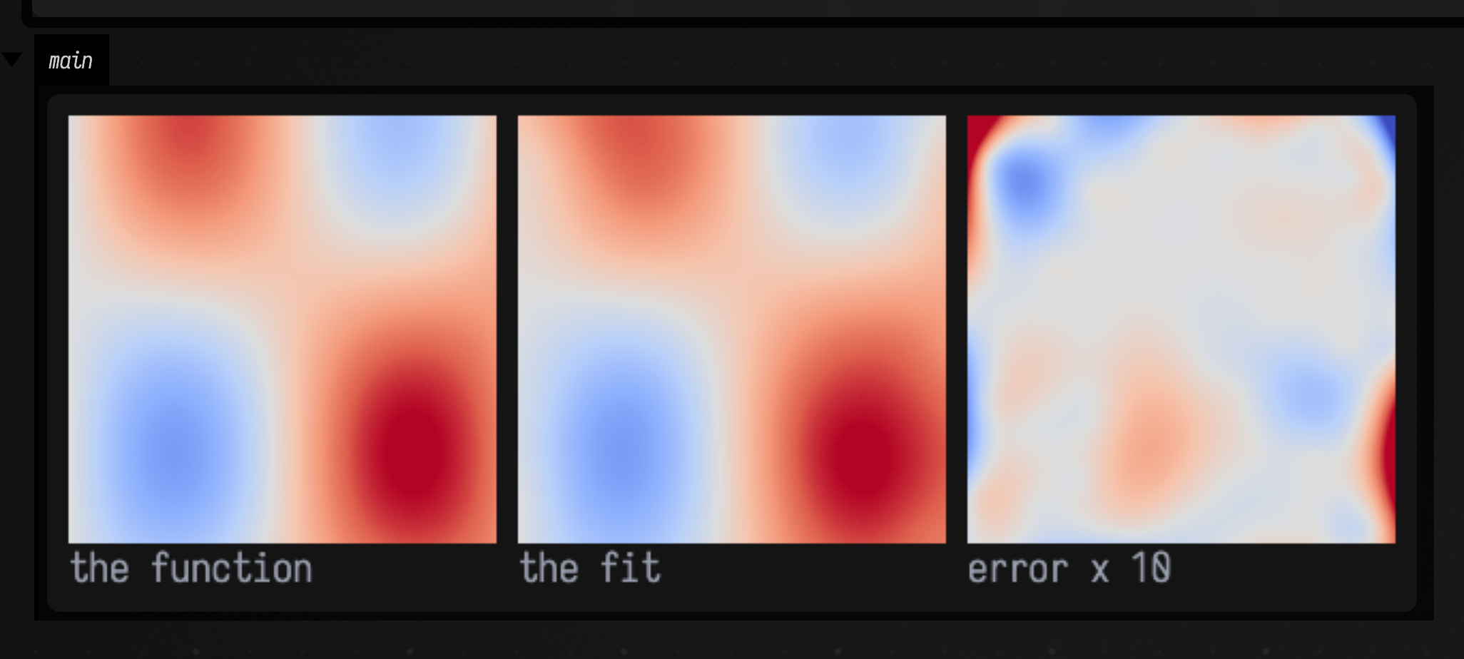
The thin-plate kernel is the default because it has no shape parameter to get wrong. With it the field
also fits a plane alongside the kernels (trend = true), so a tilted plane through the samples comes
back exactly and the kernels only describe the departures from it. A kernel with a width, like
RbfKernels.gaussian(2.0), can do better when the width suits the data, and leaveOneOutRmse() is how
to tell: it is how far each sample is from what the other 59 predict there, computed without
refitting. Here the gaussian's 0.043 beats the thin plate's 0.100. smoothing stops the surface
passing exactly through the samples, for noisy data, and RbfField(dimension) with add and
removeAt builds one sample at a time, in any number of dimensions.
Timeline, granular, and stream filters
spliceWindow
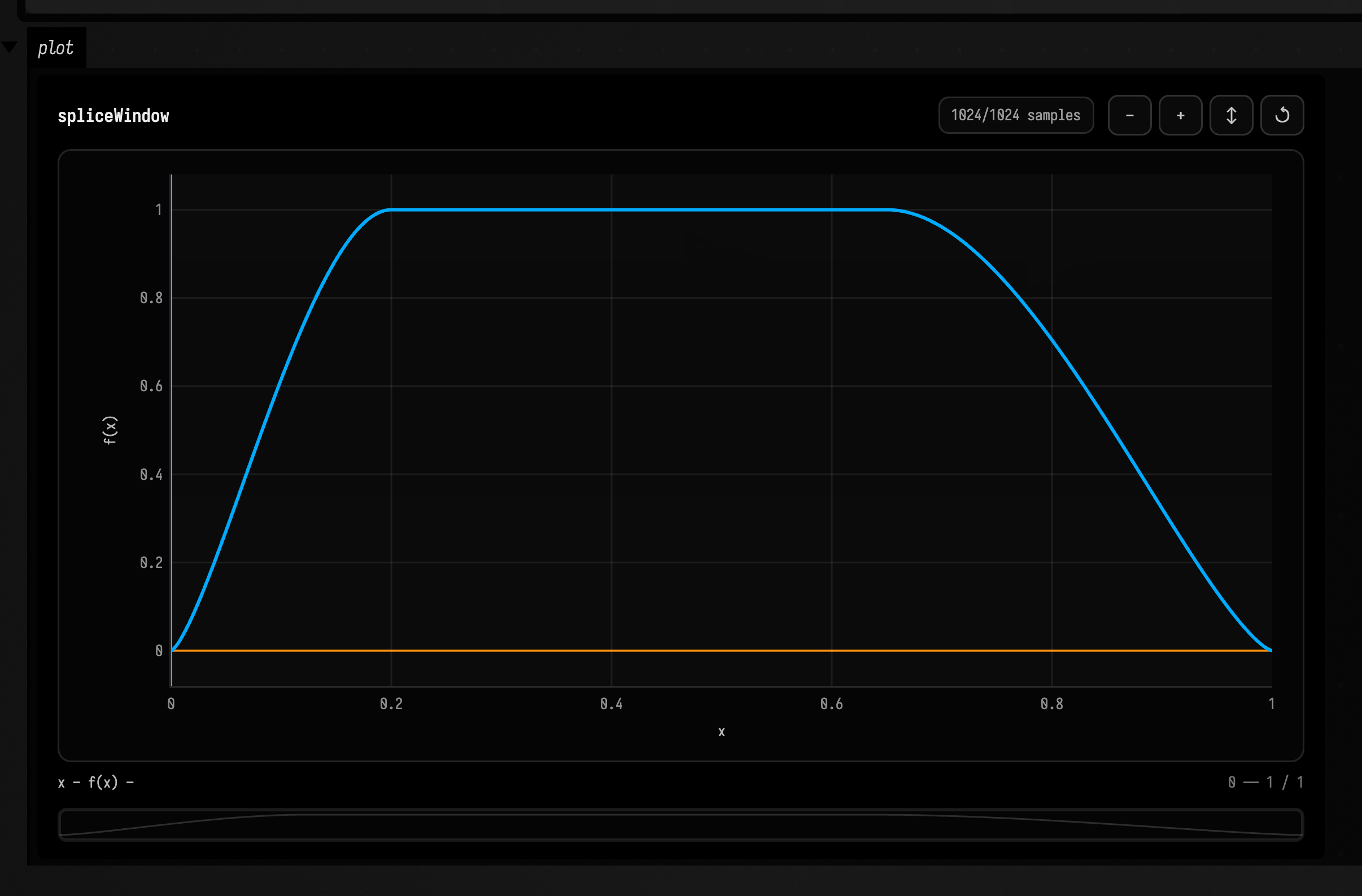
spliceWindow creates fade weights for joins and overlaps.
Simple
Makes a fade-in/fade-out window for splicing a chunk into a timeline.
val w = spliceWindow(fadeIn = 0.1, fadeOut = 0.1)Creative
:::static
with(Functions) {
    val w = spliceWindow(0.2, 0.35).pow(constant(0.7))
    w.plot()
}
timelineGraph / timeline
Timeline builders place functions as chunks that can overlap, repeat, or be stretched.
Simple
Builds a one-chunk timeline graph from a placed sine function.
val t = timeline {
    sin(2.0).place()
}
Creative
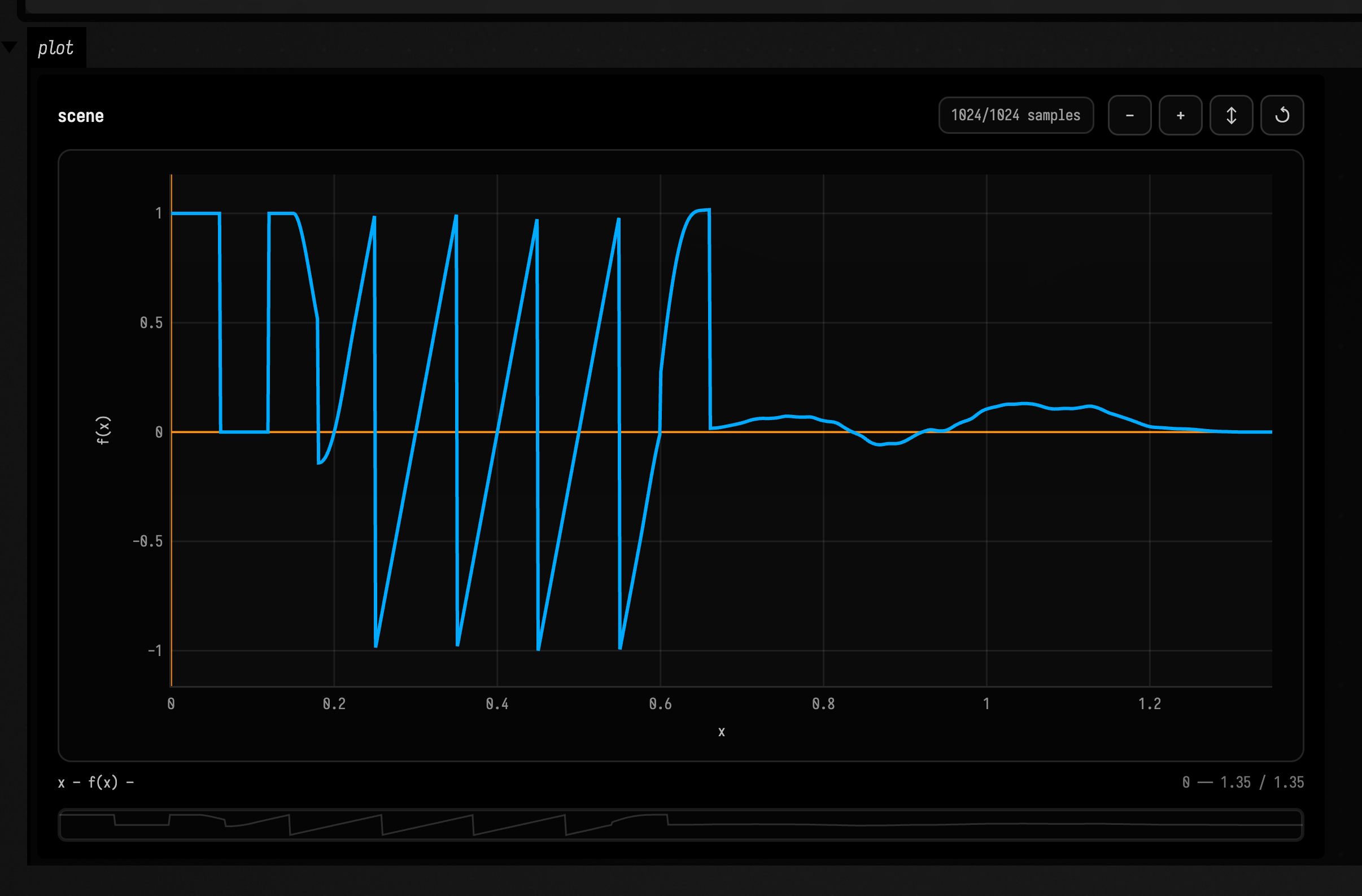
:::static
with(Functions) {
    val t = timeline(name = "scene") {
        mark("start")
        pulseTrain(0.12).place(duration = 0.7, mapMode = Functions.ChunkMapMode.WRAP)
        fbm(4, 3.0, 0.35).overlap(amount = 0.15, duration = 0.8, blend = ADD)
        moveToMark("start", 0.35)
        saw(0.2).splice(lookBack = 0.2, duration = 0.5)
    }
    t.plot()
}
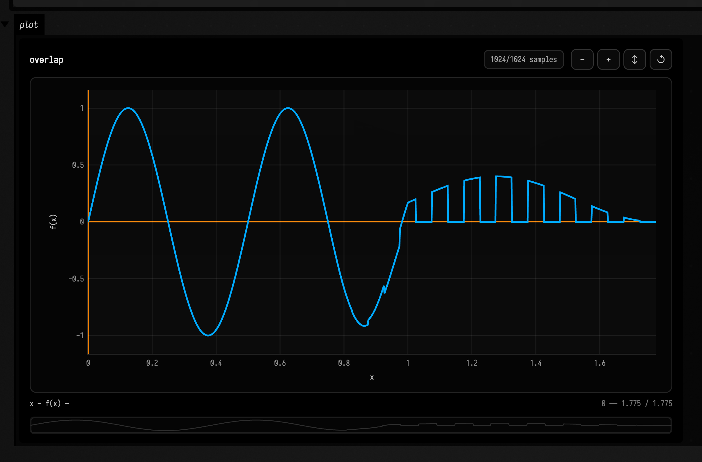
then / overlapping / overlapWith
Composition operators concatenate or crossfade functions along a timeline.
Simple
Places the saw after the sine, producing a two-part phrase.
val phrase = (sin(2.0) over (0.0..1.0)) then (saw(0.15) over (0.0..1.0))Creative
:::static
with(Functions) {
    val phrase = ((sin(2.0) over (0.0..1.0)) overlapping ramp(0.05, 0.25)) with (pulseTrain(0.1) / gain(0.4))
    val same = sin(2.0).overlapping(0.25, saw(0.15))
    phrase.plot()
}
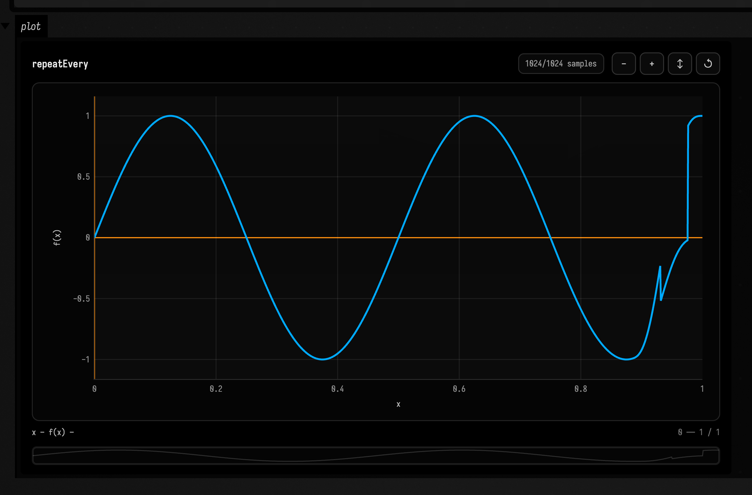
List.sequence / palindrome / roundRobin
List combiners arrange multiple functions into ordered, mirrored, or cycling phrases.
Simple
Concatenates the list of functions with a small overlap between neighbors.
val phrase = [sin(2.0), saw(0.12), square(0.18)].sequence(overlap = 0.05)Creative
:::static
with(Functions) {
    val cycle = [sin(2.0), pulseTrain(0.09), fbm(3, 4.0, 0.4)].palindrome(overlap = ramp(0.02, 0.12)) / repeatEvery(2.0)
    cycle.plot()
}
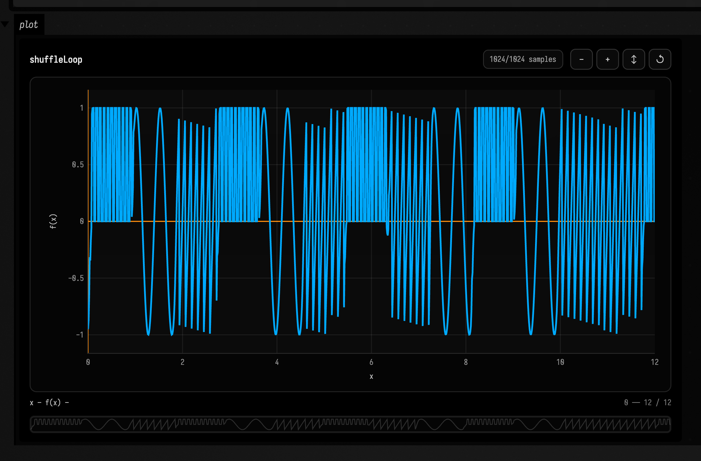
List.sequenceLoop / shuffleLoop
Looping list combiners repeat a sequence, optionally shuffled by seed.
Simple
Repeats the listed functions forever, then trims the result to 0.0..8.0.
val f = [sin(2.0), saw(0.2)].sequenceLoop() over (0.0..8.0)Creative
:::static
with(Functions) {
    val f = [sin(2.0), saw(0.13), pulseTrain(0.08)].shuffleLoop(seed = 12, overlap = 0.1) over (0.0..12.0)
    f.plot()
}
List.randomSequence / weightedSequence
Random sequence helpers choose chunks by seed, slot size, and optional weights.
Simple
Chooses random list entries in fixed-width slots, then trims to six seconds.
val f = [sin(2.0), saw(0.2)].randomSequence(seed = 3, slot = 0.4) over (0.0..6.0)Creative
:::static
with(Functions) {
    val f = [sin(2.0), saw(0.12), pulseTrain(0.08)].weightedSequence(
        [0.6, ramp(0.1, 0.35), 0.15],
        seed = 7,
        overlap = ramp(0.02, 0.08),
    ) over (0.0..10.0)
    f.plot()
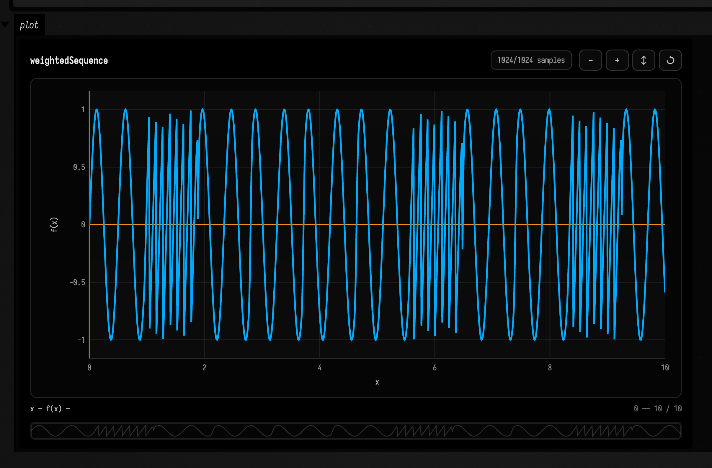
}
List.stack / average / select / morph
Stacking and selection helpers combine many functions at the same x position.
Simple
Sums the list's functions into a single stacked result.
val f = [sin(2.0), saw(0.2) * 0.3].stack()Creative
:::static
with(Functions) {
    val f = [sin(2.0), saw(0.14), fbm(3, 3.0, 0.6)].morph(ramp(0.0, 2.0))
    f.plot()
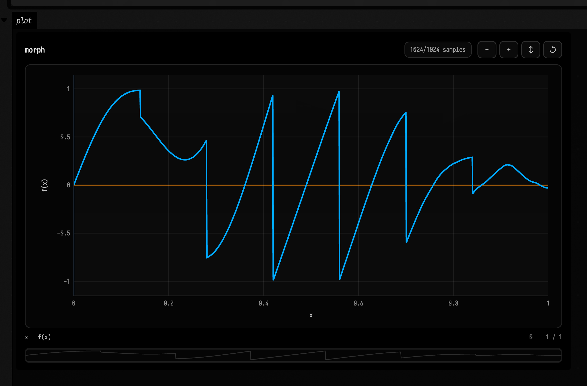
}
/ transform palette
Transform-palette helpers make compact chains of common time and value edits.
Simple
Stretches the sine across four units, then speeds up, smooths, and scales it through a transform chain.
val f = sin(3.0) / stretch(0.0..4.0) / faster(2.0) / lowPass(0.04) / gain(0.8)Creative
:::static
with(Functions) {
    val f =
        (fbm(4, 5.0, 1.0) /
            all /
            slower(ramp(0.8, 1.7)) /
            highPass(remap(0.02, 0.08)) /
            turbulence(0.02, ramp(8.0, 18.0)) /
            crush(5) /
            mirrorEvery(0.4)) over (0.0..4.0)
    f.plot()
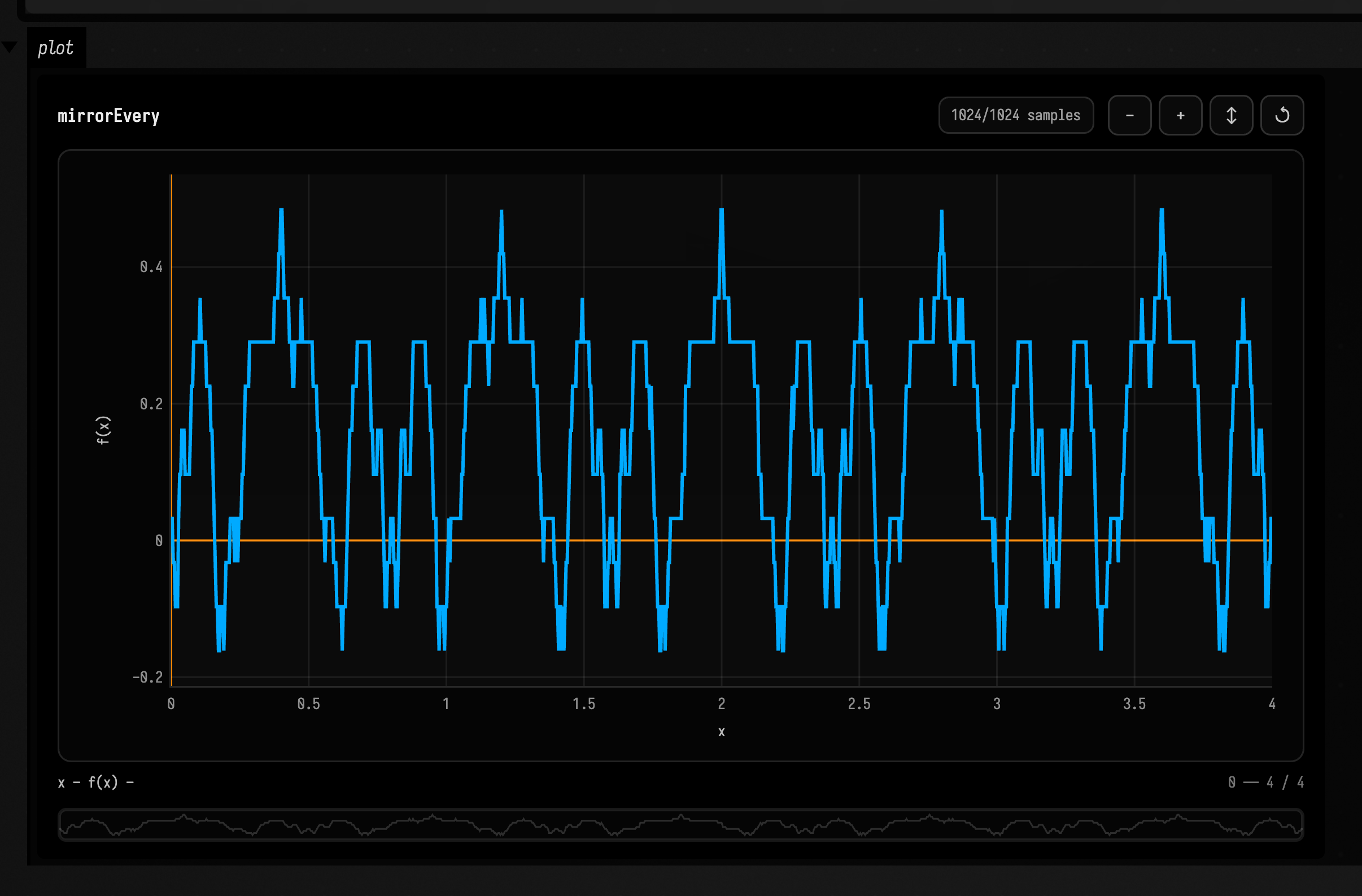
}
fold / rectify / quantize / crush / chebyshev (waveshaping)
The waveshaping / distortion transforms are the value-domain (west-coast) counterparts to the time-domain hold / stepHold pair: they reshape a signal's amplitude rather than its clock. They are ordinary FnTransform factories, so they compose in through / pipe / / chains and surface in the type-aware infix completion like every other transform.
fold(threshold)— a west-coast wavefolder. Within[-threshold, threshold]the signal passes through unchanged; each time it would cross the threshold it is reflected back into the band. The result is continuous, odd-symmetric, and always bounded to[-threshold, threshold]— unlikeclipAt, folding turns overshoot into extra harmonics instead of a flat top.rectify(mode)— half- or full-wave rectifier.RectifyMode.FULL(the default) yields|x|;RectifyMode.HALFclamps the negative excursion to zero. The mode rides as a tag on the graph node, the waywithEdgecarries itsEdgeMode.quantize(levels)— an amplitude staircase that snaps the value to exactlylevelsevenly-spaced steps across[-1, 1]: a bitcrush of the value, distinct from the time-domainstepHold.levelsis a param child.crush(bits)— a bit-crusher, the value-domain sibling ofquantize. It snaps to2^bits − 1steps across[-1, 1], so lower bit-depths sound and look coarser.bitsis a param child, andop=bitcrushis an accepted alias forop=crush.chebyshev(order)— the canonical harmonic-generating waveshaper. Pushing a unit-amplitude cosine through the order-n Chebyshev polynomial Tₙ produces the pure n-th harmonic, because Tₙ(cos θ) = cos(nθ). The input is clamped to[-1, 1]first (the standard shaper guard, as withsoftClip), and evaluated in that trig form, Tₙ(v) = cos(n·arccos v), which is exact for integer n and continuous in n. Sinceorderis a param child and can itself be anFn, a ramped order glides between harmonics.
Every member of the family (fold, rectify, quantize, crush, chebyshev, alongside clip/softClip/clamp/wrapY) is a rebuildable node(...) carrying an OpSpec in OpRegistry, rather than an opaque mapY lambda. So the graph-rewrite, evolve, and transmutation machinery can swap any of them in by name: op=rectify, op=quantize, op=crush, and the rest.
Simple
Folds the ramp back on itself past 0.7, so the rising line becomes a triangle bounded to [-0.7, 0.7].
val f = (ramp(-2.0, 2.0) over (0.0..1.0)) / fold(0.7)Creative
:::static
with(Functions) {
    // A loud sine, folded then rectified then staircased — a full distortion chain.
    val f = (sin(3.0) * 1.6 / fold(0.7) / rectify() / quantize(8)) over (0.0..2.0)
    f.plot("waveshaped")
    // Compare the shapes produced by applying each shaper to the same sine samples.
    val sweep = ((sin(0.5) * 2.0) over (0.0..2.0))
    (sweep / fold(0.6)).plot("fold(0.6)")
    (sweep / quantize(5)).plot("quantize(5)")
    // Chebyshev turns a clean sine into its pure n-th harmonic.
    ((sin(1.0) over (0.0..2.0)) / chebyshev(3)).plot("chebyshev(3) — 3rd harmonic")
}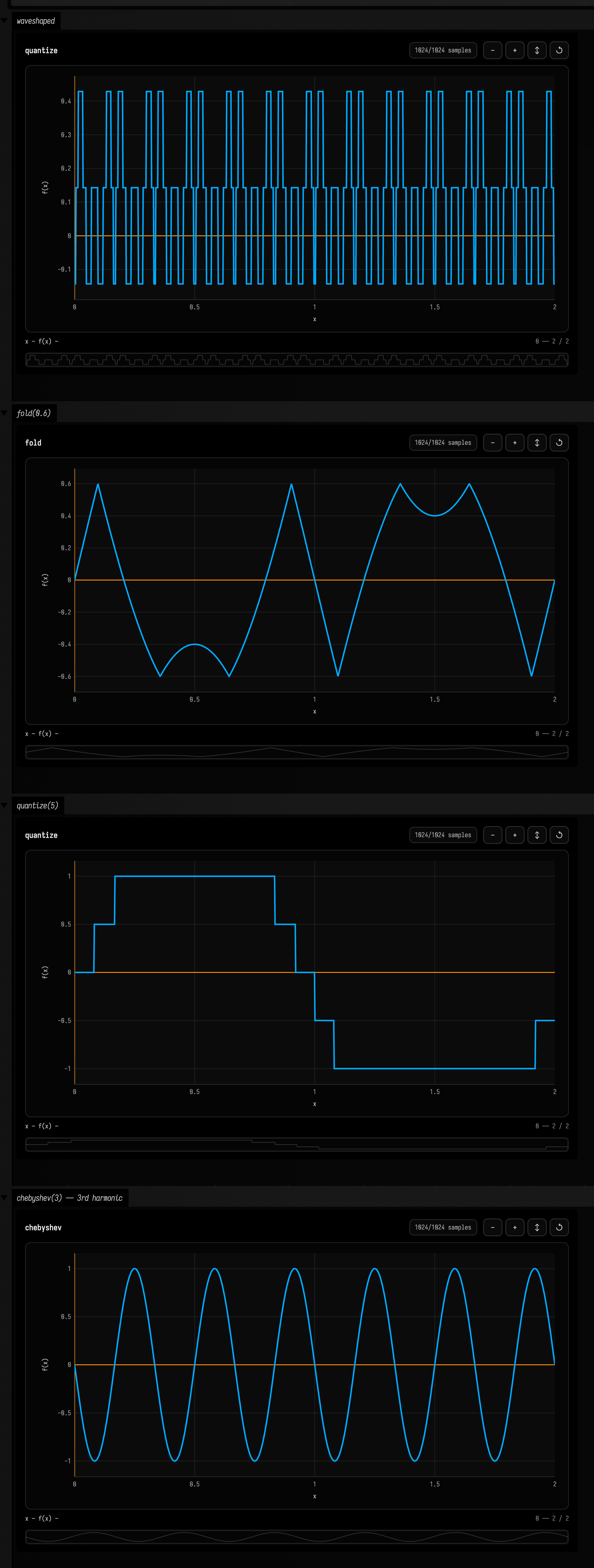
The transfer curves. Sweeping a ramp -2..2 through each shaper and plotting the result against x draws that shaper's transfer curve directly: the shape it imposes on its input. The montage below runs the whole waveshaper family (fold / rectify / quantize / crush / chebyshev / clip / softClip / clamp / wrapY) live in a Field box. Each is a pure value shaper, so the curves come out the same on every run.
:::static
with(Functions) {
    // A ramp sweeping -2..2 across the window: plotting a shaper of it against x draws
    // that shaper's transfer curve directly — the shape it imposes on its input.
    val sweep = ramp(-2.0, 2.0) over (0.0..1.0)
    sweep.withName("input sweep -2..2").plot(channel = "sweep", title = "input: ramp -2..2", heightPx = 150)
    (sweep / fold(0.7)).plot(channel = "fold", title = "fold(0.7) — wavefolder triangle", heightPx = 150)
    (sweep / rectify(Functions.RectifyMode.FULL)).plot(
        channel = "rectFull",
        title = "rectify(FULL) — |x|",
        heightPx = 150,
    )
    (sweep / rectify(Functions.RectifyMode.HALF)).plot(
        channel = "rectHalf",
        title = "rectify(HALF) — max(0, x)",
        heightPx = 150,
    )
    (sweep / quantize(6)).plot(channel = "quant", title = "quantize(6) — staircase", heightPx = 150)
    (sweep / crush(3)).plot(channel = "crush", title = "crush(3) — bit-depth steps", heightPx = 150)
    (sweep / chebyshev(3)).plot(channel = "cheb", title = "chebyshev(3) — T₃ (clamps to [-1, 1])", heightPx = 150)
    sweep.clip(0.8).plot(channel = "clip", title = "clip(0.8) — hard rails", heightPx = 150)
    sweep.softClip(3.0).plot(channel = "soft", title = "softClip(3.0) — tanh knee", heightPx = 150)
    sweep.clamp(-0.8, 0.8).plot(channel = "clamp", title = "clamp(-0.8, 0.8)", heightPx = 150)
    sweep.wrapY(-0.8, 0.8).plot(channel = "wrap", title = "wrapY(-0.8, 0.8) — sawtooth wrap", heightPx = 150)
}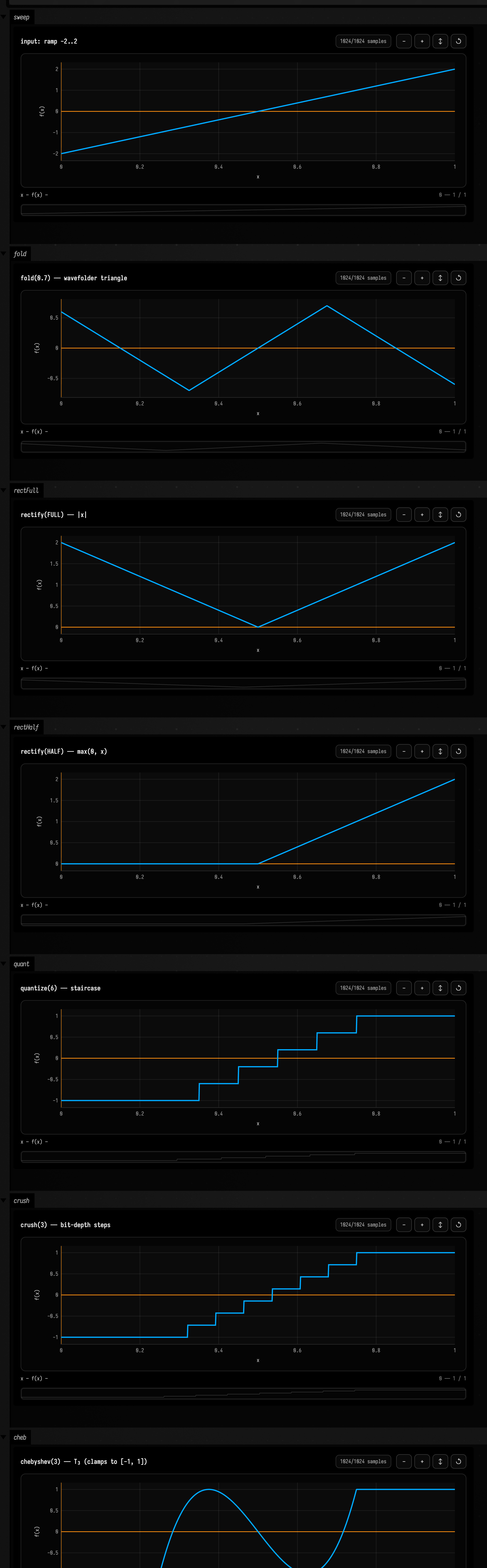
Replay it live. A loadable operation transcript, assets/functions/waveshape-transforms.operations.yaml, builds and plots the whole family in a fresh Field document. Replay it with field_backdoor.py --scratch (macro write … && macro run …) or hand the YAML to the field_run_transcript MCP tool. See Automating Field for the transcript path. A companion transcript, assets/functions/chebyshev-waveshaper.operations.yaml, builds the two boxes captured below. A third, assets/functions/waveshaper-family-evolvable.operations.yaml, plots rectify/quantize/crush and then transmutes a clipped sine into each of them by name through the rewrite DSL (clip => op=rectify, op=quantize, op=crush), which is the same op vocabulary the evolve loop mutates over. Without a Field at all, WaveshapeWorkedExample runs the same geometry on the CPU as a jvm-main smoke and a JUnit test.
The harmonic ladder. A single-cycle sine, then the same sine pushed through chebyshev(2..5), where each output is the pure n-th harmonic since Tₙ(cos θ) = cos(nθ). Finally an order = ramp(1.0, 6.0) sweep glides continuously from the 1st up to the 6th harmonic across the window, order being a real number rather than a stepped integer.
:::static
with(Functions) {
    val fundamental = sin(1.0) over (0.0..1.0)
    fundamental
        .withName("fundamental (harmonic 1)")
        .plot(channel = "fund", title = "input: sine, 1 cycle", heightPx = 150)
    (fundamental / chebyshev(2)).plot(channel = "h2", title = "chebyshev(2) — 2nd harmonic", heightPx = 150)
    (fundamental / chebyshev(3)).plot(channel = "h3", title = "chebyshev(3) — 3rd harmonic", heightPx = 150)
    (fundamental / chebyshev(4)).plot(channel = "h4", title = "chebyshev(4) — 4th harmonic", heightPx = 150)
    (fundamental / chebyshev(5)).plot(channel = "h5", title = "chebyshev(5) — 5th harmonic", heightPx = 150)
    // order is an Fn, so a value ramp 1..6 sweeps the harmonic across the window.
    fundamental
        .chebyshev(ramp(1.0, 6.0) over (0.0..1.0))
        .plot(channel = "sweep", title = "chebyshev(order = ramp 1..6) — harmonic sweep", heightPx = 160)
}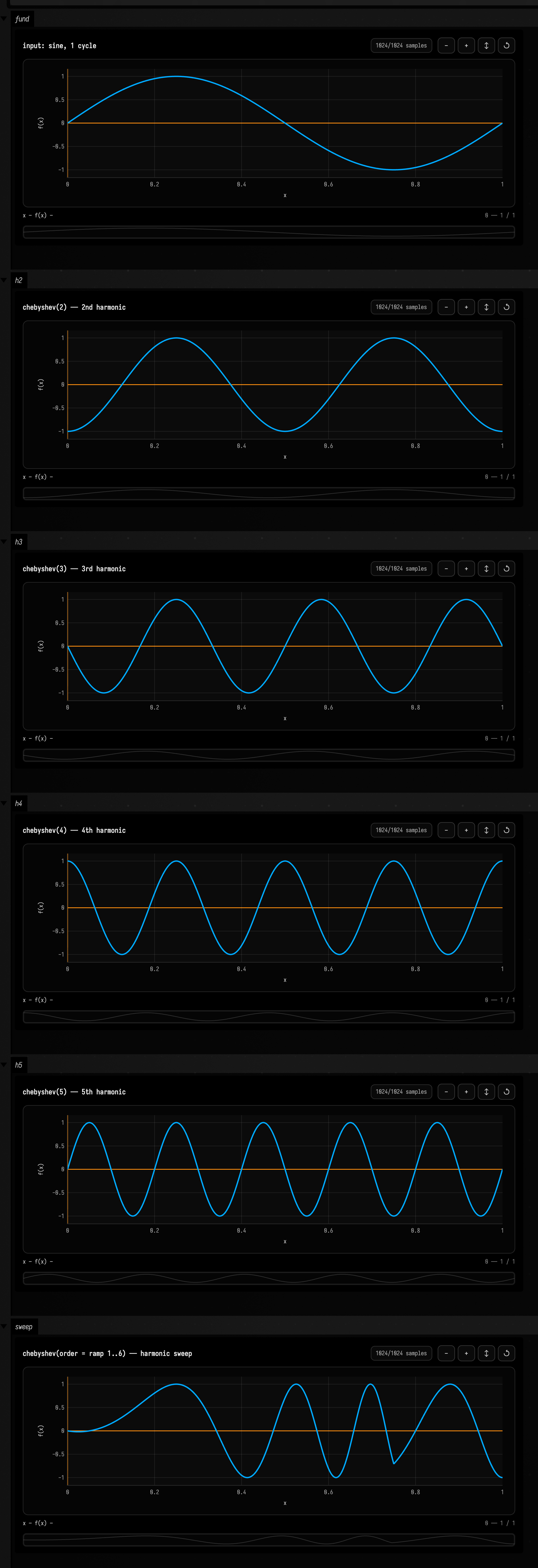
Because a waveshaper reshapes amplitude, chebyshev colours any bounded signal, not just a clean oscillator. The transcript's second box feeds band-limited Perlin noise through chebyshev(2/3/5): T₂ folds the noise toward the rails, and higher orders multiply its zero-crossings.
:::static
with(Functions) {
    // Amplified toward [-1, 1] so the shaper has full range (chebyshev clamps internally).
    val noise = perlinNoise(seed = 7L, frequency = 6.0, amplitude = 1.6) over (0.0..1.0)
    noise.withName("perlin noise").plot(channel = "n", title = "input: perlin noise (freq 6)", heightPx = 150)
    (noise / chebyshev(2)).plot(channel = "n2", title = "perlin / chebyshev(2)", heightPx = 150)
    (noise / chebyshev(3)).plot(channel = "n3", title = "perlin / chebyshev(3)", heightPx = 150)
    (noise / chebyshev(5)).plot(channel = "n5", title = "perlin / chebyshev(5)", heightPx = 150)
}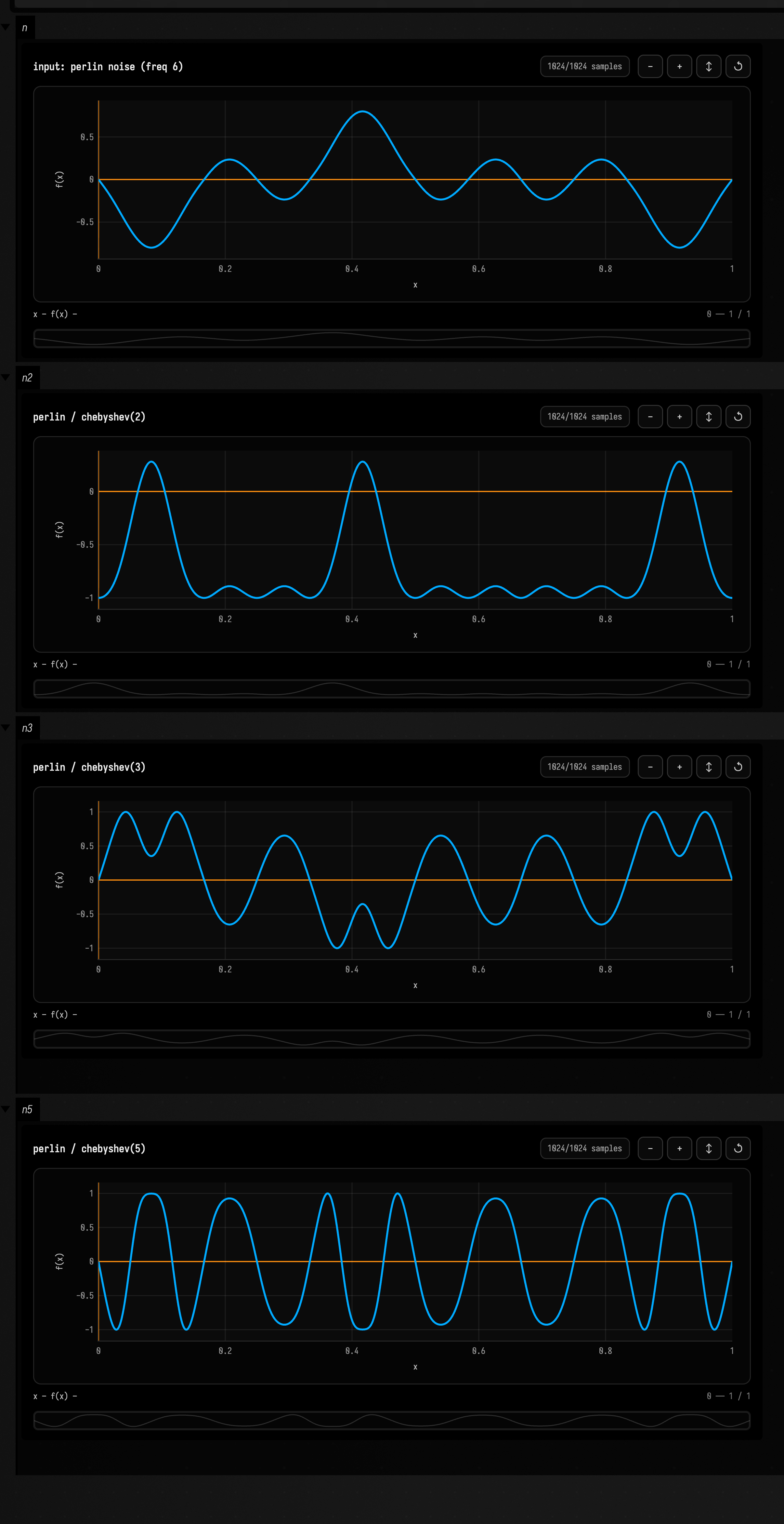
copyPaste / randomRepeat / randomCopyPaste
Copy and repeat transforms reuse source fragments deterministically or randomly.
Simple
Copies the 0.1..0.3 slice of the sine wave into 0.7..0.9.
val f = sin(3.0) / copyPaste(0.1..0.3, 0.7..0.9)Creative
:::static
with(Functions) {
    val f =
        (pulseTrain(0.08) /
            randomRepeat(period = ramp(0.12, 0.28), seed = 4) /
            randomCopyPaste(grain = ramp(0.04, 0.12), seed = 8, density = ramp(0.35, 0.85))) over (0.0..6.0)
    f.plot()
}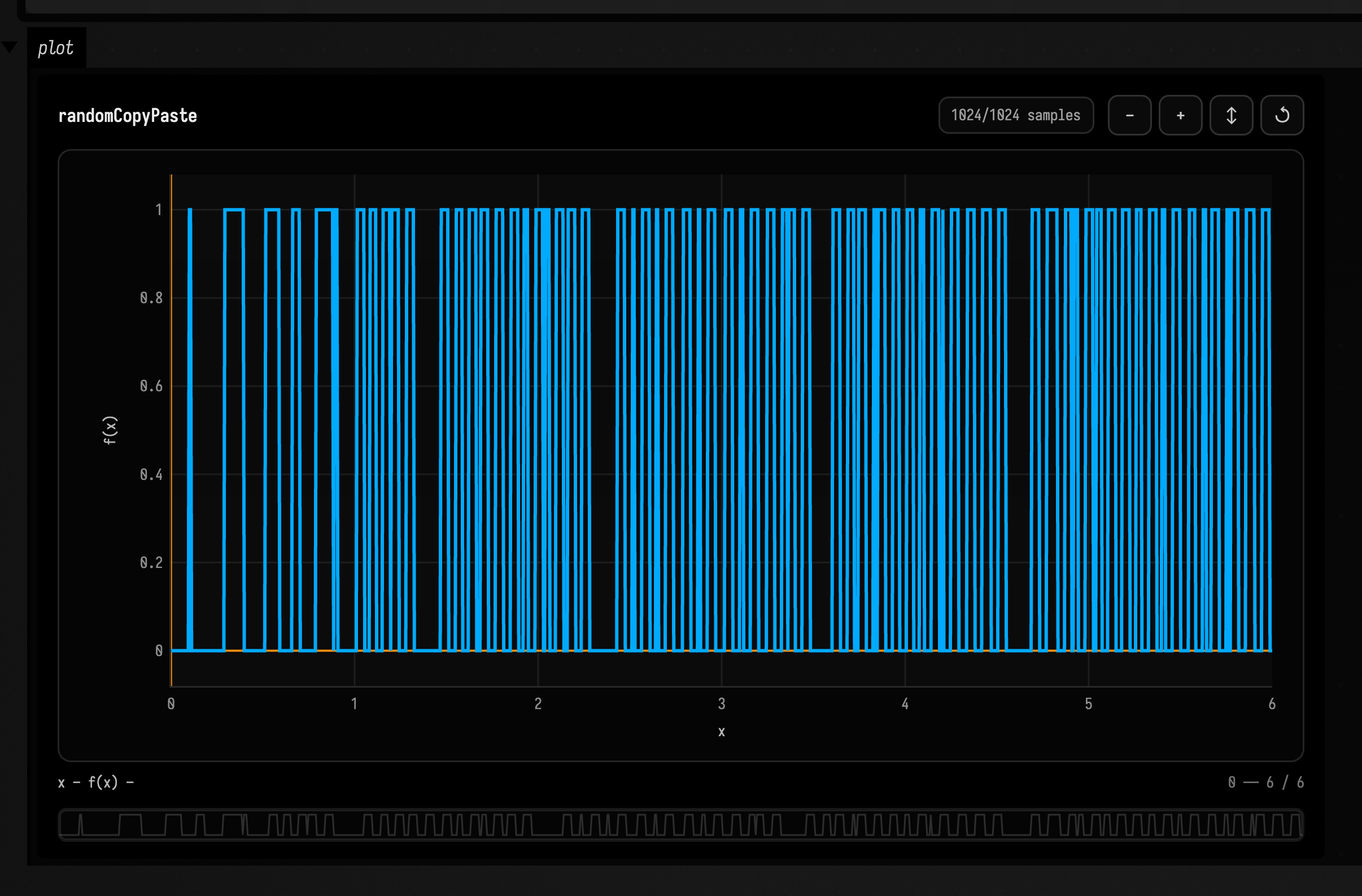
repeatToFit / stretchToFit / snapshot / lookBack
Timeline utilities fit sources to durations or reuse recently placed material.
Simple
Fills a two-unit timeline span by repeating the source function.
val g = timelineGraph {
    repeatToFit(sin(2.0), duration = 2.0)
}
Creative
:::static
with(Functions) {
    val g = timelineGraph {
        stretchToFit(fbmPerlin(2, 2.0, 1.0), duration = 3.0)
        val ghost = snapshot(offset = 0.12)
        ghost.place(duration = 1.5, blend = ADD, gain = 0.4)
    }
    g.asFn("snapshot").plot()
}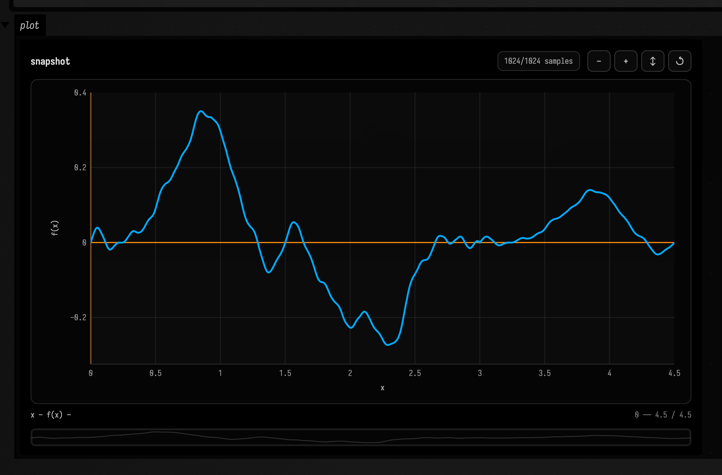
granular
granular resynthesizes a function from small overlapping source grains.
Simple
Rebuilds the sine wave from overlapping short grains.
val f = sin(3.0).granular(grainSize = 0.05, spacing = 0.04)Creative
:::static
with(Functions) {
    val f =
        fbmPerlin(1, 3.0, 0.8)
            .granular(
                grainSize = 0.04,
                spacing = 0.027,
                jitter = 0.35,
                overlap = 2,
                seed = 3,
                window = gaussianWindow(0.0..1.0, 0.3),
            )
    f.plot()
}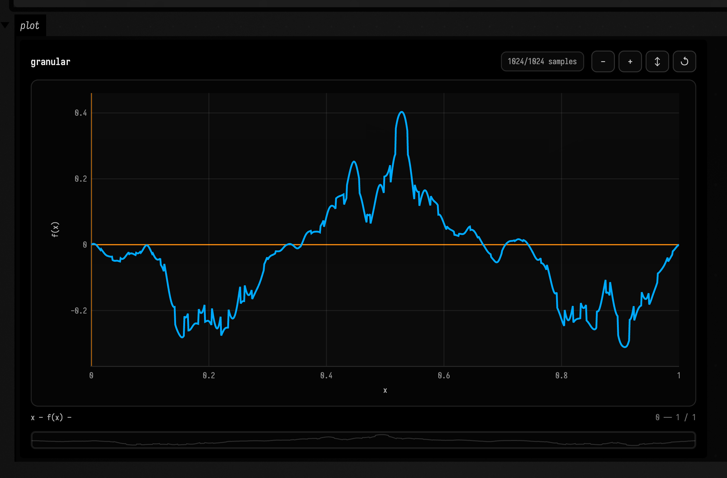
lowpassStream / highpassStream
Stream filters process sampled values lazily for lightweight smoothing or edge emphasis.
Simple
Streams low-pass filtered sine samples into a list.
val s = sin(2.0).lowpassStream(alpha = 0.2).take(64).toList()Creative
:::static
with(Functions) {
    val s = (pulseTrain(0.12) + valueNoise(5, 22.0, 0.2)).highpassStream(alpha = 0.88, step = 0.004).take(256).toList()
    val f = s.toFn(domain = 0.0..1.0).withName("highpassStream")
    f.plot()
}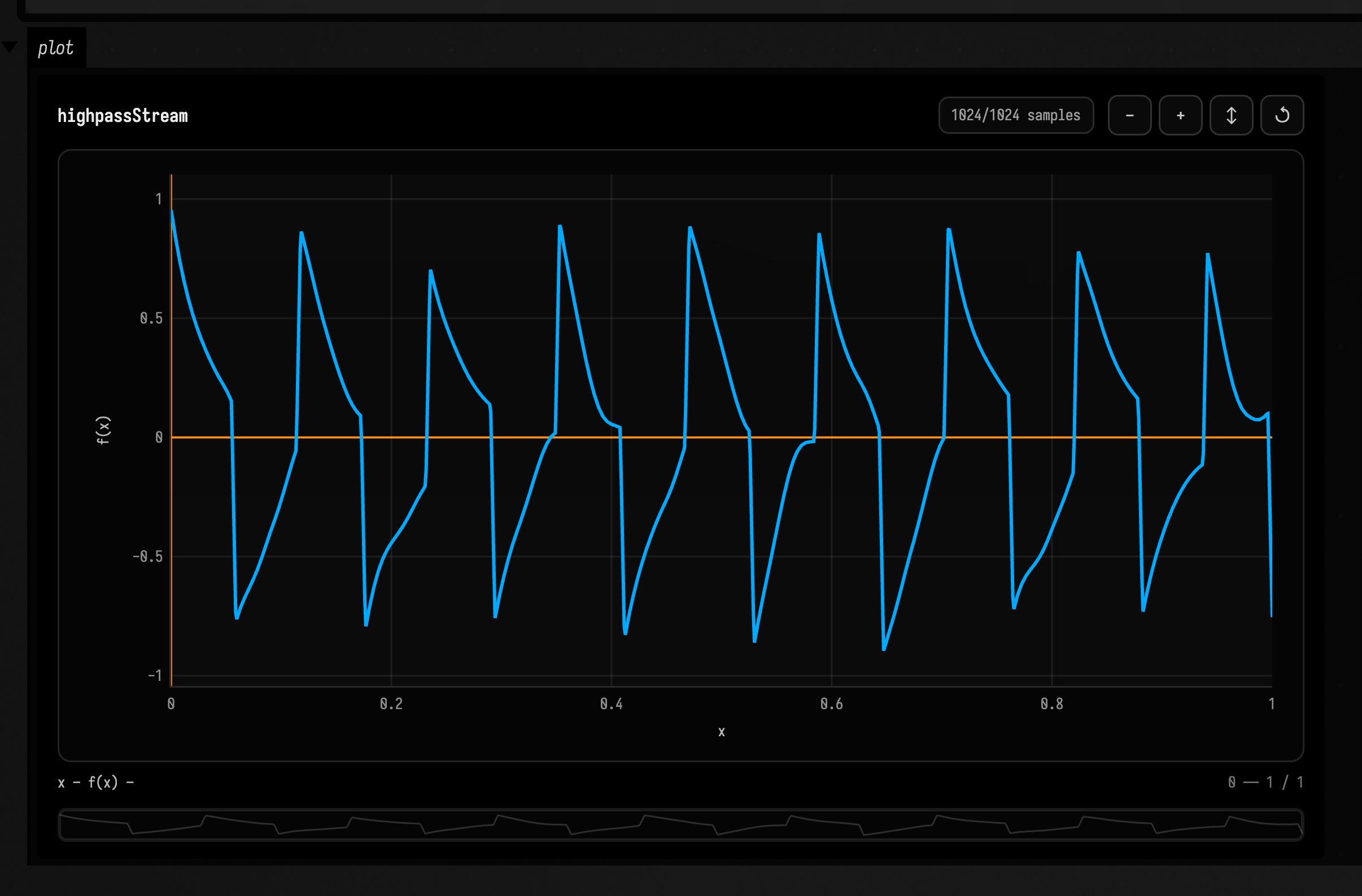
demo
demo builds a compact bundle of representative series and statistics for quick validation.
Simple
Runs the built-in demo over the default domain and returns sampled result data.
val result = demo(sampleCount = 256)Creative
:::static
with(Functions) {
    val result = demo(sampleCount = 1024, seed = 77, domain = -0.25..1.25, printSummary = false)
    val series = result.series.first { it.name == "mixed" }
    val f = series.ys.toFn(domain = series.domain, interpolation = CUBIC).withName("demo mixed")
    f.plot()
}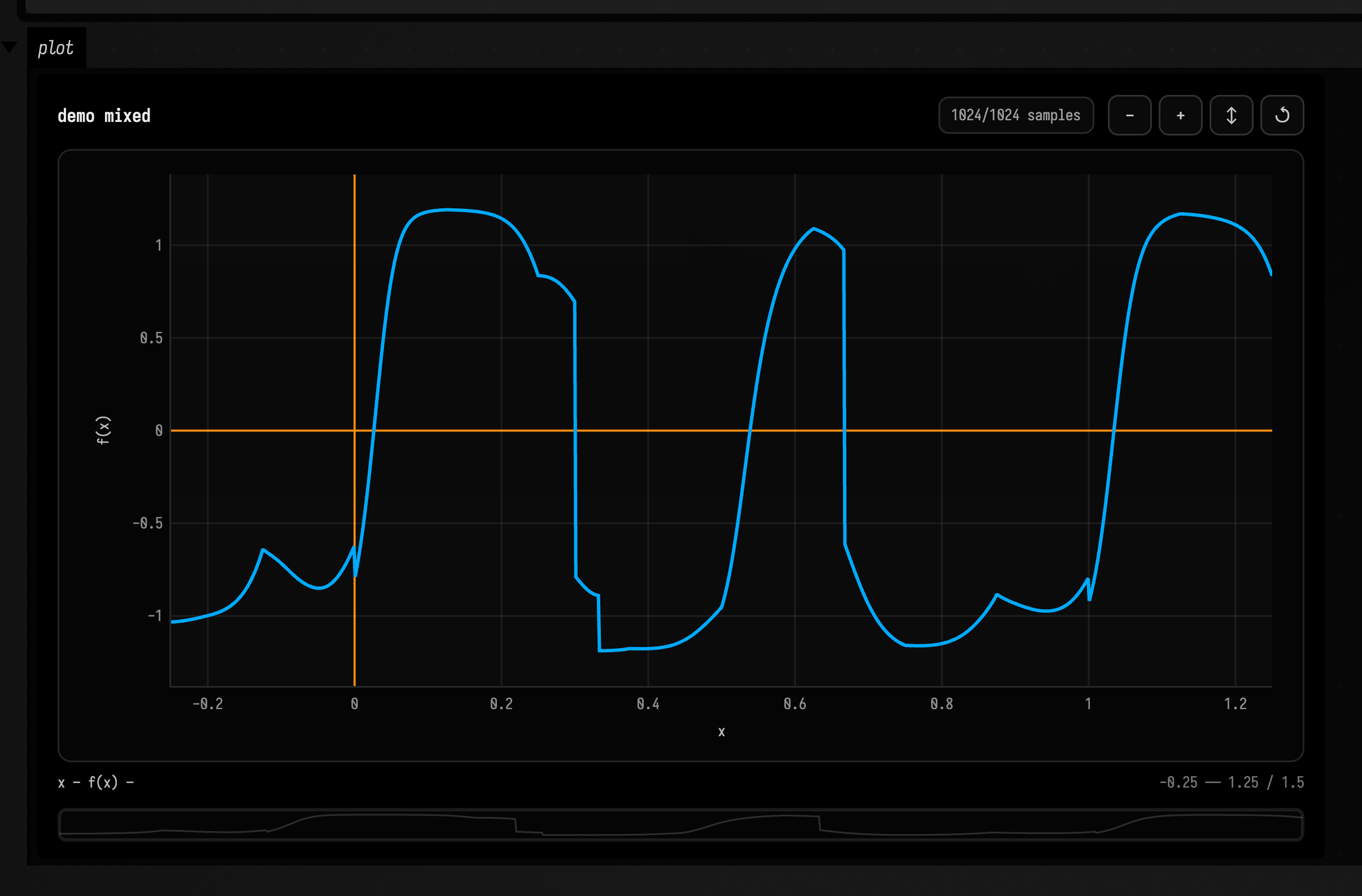
Complete API addendum: utility classes and methods
The sections above cover the primary signal-shaping API. This addendum closes the remaining symbol gaps with plain examples and more developed variants.
Domain methods
These entries cover interval operations used to build, trim, and remap Fn domains. In this subsection, d means domain(0.0..1.0).
Range notation / point / centered
Domain helpers create and combine numeric intervals for construction and sampling.
Simple
Creates numeric domains with terse range notation and uses them directly in functions.
val a = 0.0..1.0
val b = sin(5, domain = 0..1)
Creative
val a = Functions.Domain.centered(0.5, 0.42).intersect(domain(0.0..1.0))

// → Domain(0.08..0.92)
containsInclusive / contains
Containment checks ask whether an x value lies inside a domain.
Simple
Reports that 0.2 lies inside the domain.
val inside = d.containsInclusive(0.2) // → trueCreative
val mask = if (d.contains(0.77)) one() else zero() // 0.77 is inside → one()expand / shrink
Expansion and shrinking grow or contract a domain around its endpoints.
Simple
Widens the domain by 0.1 on both sides.
val wide = d.expand(0.1) // → Domain(-0.1..1.1)Creative
val band = d.expand(0.2).shrink(0.05) // → Domain(-0.15..1.15)shift / scale
Domain shifts and scales move or zoom intervals without sampling an Fn.
Simple
Shifts the whole domain forward by 0.15.
val moved = d.shift(0.15) // → Domain(0.15..1.15)Creative
val zoom = d.scale(0.5, about = d.center).shift(0.1) // → Domain(0.35..0.85)lerp / alphaOf
Interpolation helpers convert between normalized alpha and concrete x positions.
Simple
Returns the point one-quarter of the way across the domain.
val x = d.lerp(0.25) // → 0.25 (a quarter across 0..1)Creative
// alphaOf(0.42) → 0.42; smoothStep eases that alpha before sampling
val warpedAlpha = smoothStep(0.0, 1.0).eval(domain(0.0..1.0).alphaOf(0.42))
clamp / wrap / reflect
Domain edge helpers keep x values inside an interval by clamping, wrapping, or reflecting.
Simple
Clamps an outside value back to the domain's upper edge.
val x = d.clamp(1.2) // → 1.0 (pulled back to the upper edge)Creative
val pingPong = d.reflect(2.7) // → 0.7 (folded back into 0..1)intersect / union
Domain set operations find overlap or coverage across intervals.
Simple
Computes the overlapping interval between d and 0.2..0.7.
val i = d.intersect(domain(0.2..0.7)) // → Domain(0.2..0.7)Creative
val merged = d.union(domain(-0.3..0.3)).intersect(domain(-0.1..0.9)) // → Domain(-0.1..0.9)Fn lifecycle and safety
These entries cover direct sampling, safe edge behavior, and lightweight relabeling of existing functions.
eval / invoke
Evaluation samples a function at one x value, either explicitly or with call syntax.
Simple
Evaluates the sine wave directly at x = 0.5.
val y = sin(2.0).eval(0.5)Creative
val y = (fbm(3, 4.0, 0.6))(0.37)evalSafe
evalSafe samples with an outside-domain policy instead of assuming x is valid.
Simple
Safely returns the outside value when sampling beyond the domain.
val y = sin(2.0).evalSafe(2.0, outside = 0.0)Creative
val y = saw(0.1).evalSafe(-0.3, edge = Functions.EdgeMode.MIRROR)over / withDomain / withName
Lifecycle helpers relabel a function with a new interval or display name. Prefer over (...) in user code; withDomain(...) is the lower-level method behind it.
Simple
Renames the sine wave to lead while preserving its behavior.
val f = sin(2.0).withName("lead")Creative
:::static
with(Functions) {
    val f = ((valueNoise(4, 12.0, 0.5) over (0.1..0.9)) / all).withName("noise-bed")
    f.plot()
}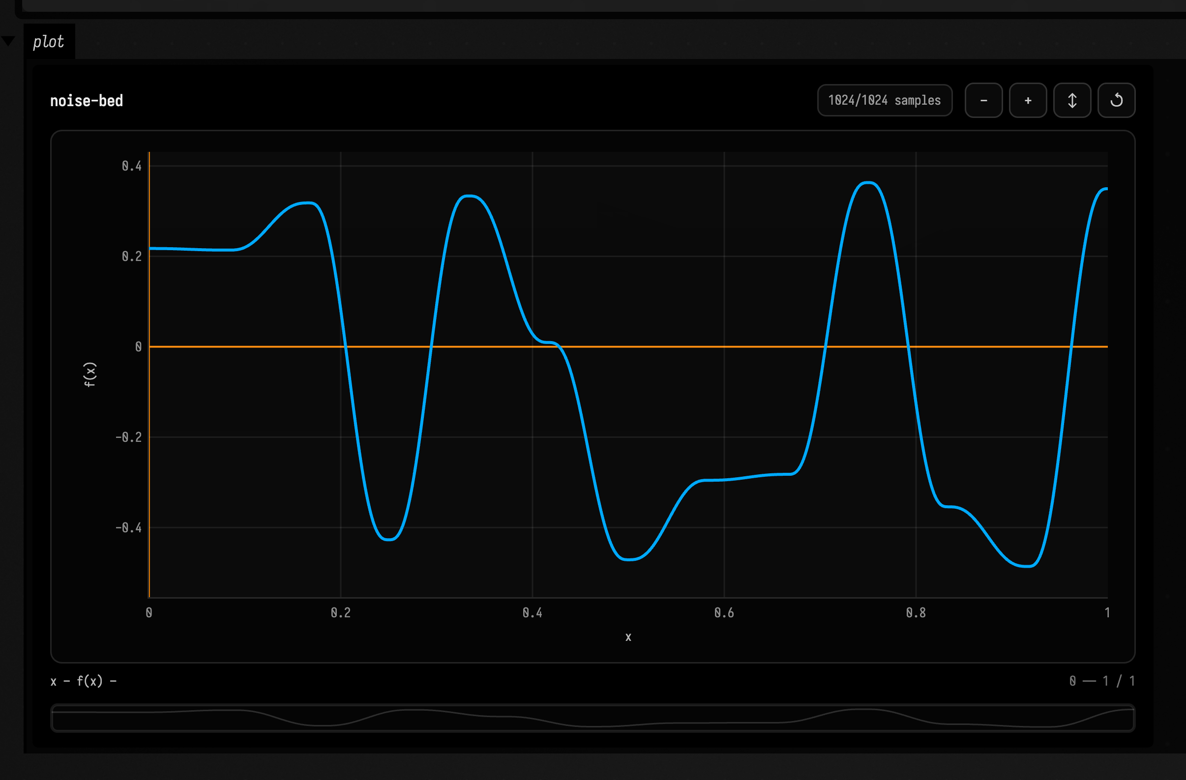
FunctionCursor methods
Cursor entries show how to pull sequential samples from an Fn when array or stream helpers are too indirect.
next()
next() advances a cursor by one step and returns the sampled value.
Simple
Advances the cursor once and returns the first sampled value.
val cur = sin(2.0).cursor(0.0, 0.01)
val y = cur.next()
Creative
:::static
with(Functions) {
    val cur = fbm(5, 3.0, 0.7).cursor(0.0, 0.002)
    repeat(32) { cur.next() }
    val f = cur.next(512).toFn(domain = 0.0..1.0, interpolation = CUBIC).withName("cursor next")
    f.plot()
}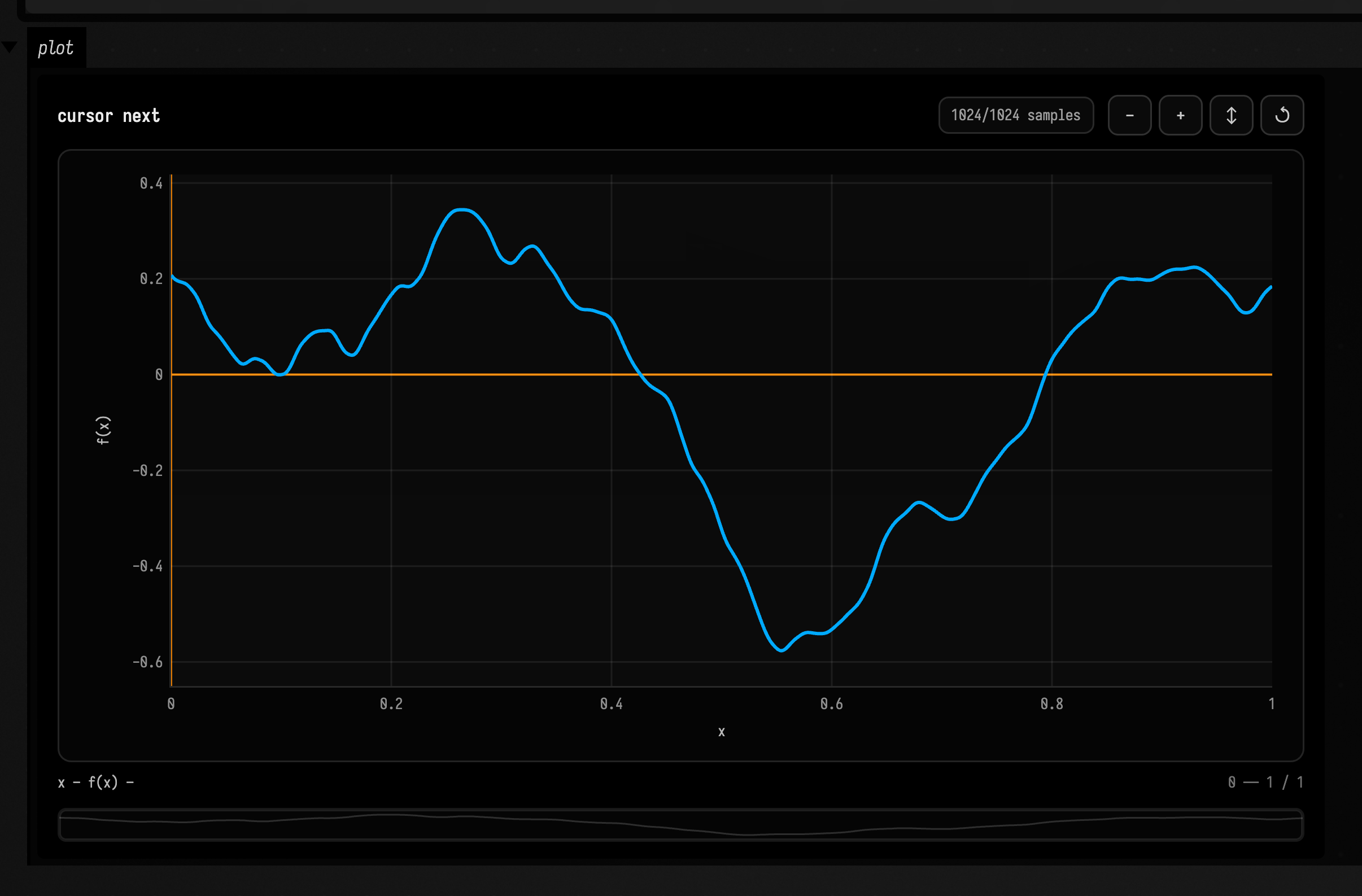
next(count)
next(count) pulls a fixed-size batch from a cursor.
Simple
Returns the next sixteen cursor samples as a batch.
val ys = sin(2.0).cursor().next(16)Creative
:::static
with(Functions) {
    val ys = pulseTrain(0.15).cursor(start = 0.25, step = 0.003).next(1024)
    val f = ys.toFn(domain = 0.0..1.0, interpolation = NEAREST).withName("cursor batch")
    f.plot()
}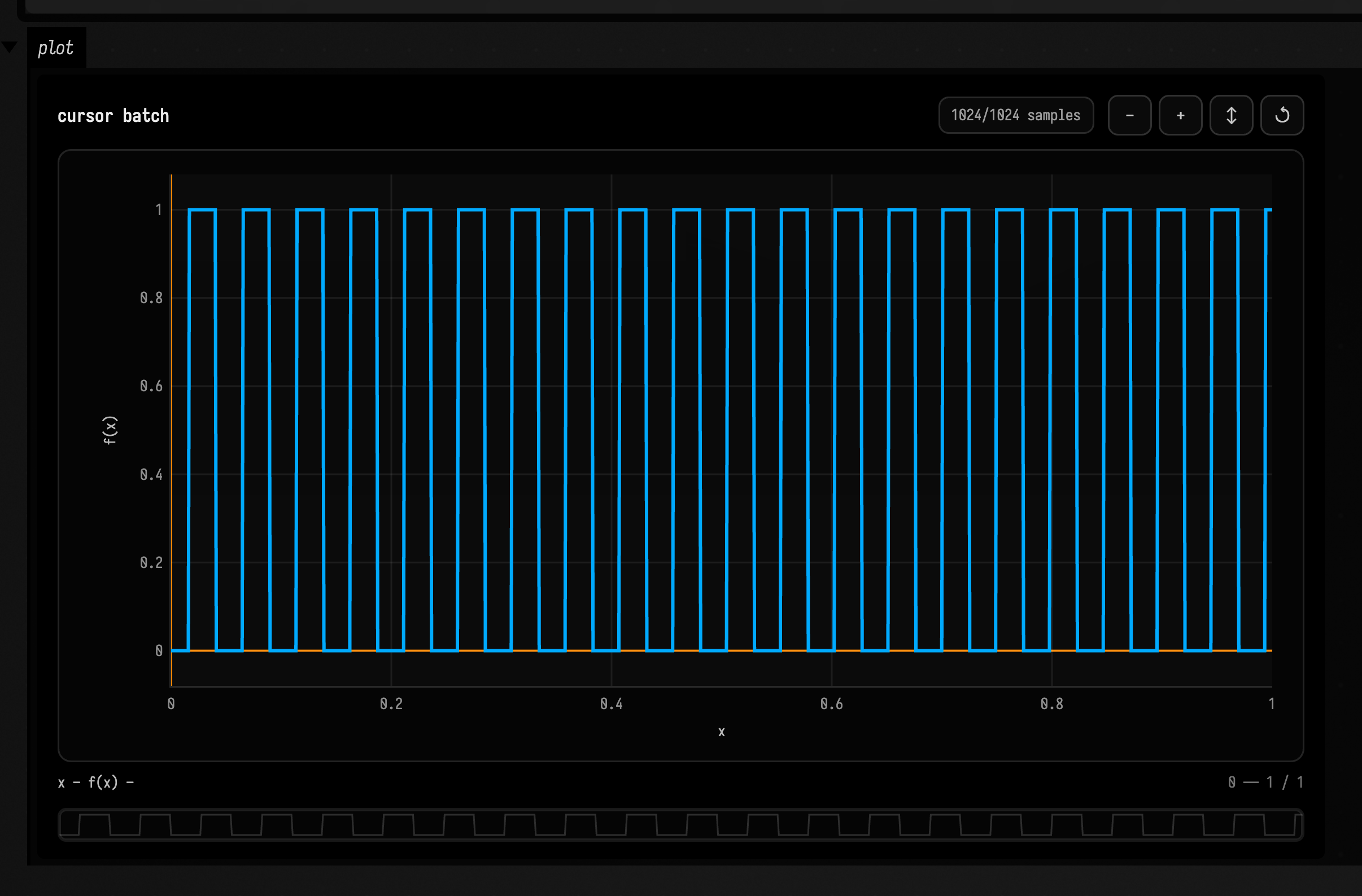
For hand-driven procedural loops, cursors also provide:
| Method | Meaning |
|---|---|
peek() |
Samples the current coordinate without advancing the cursor. Repeated peeks therefore read the same position. |
nextWithX() |
Returns both the coordinate and its sampled value, then advances. Use it when the sample needs its position attached. |
skip(count) |
Moves forward by the requested number of cursor steps without evaluating the function. It changes position without producing samples. |
seek(x) |
Moves the cursor to an absolute coordinate. The next sample comes from that position. |
reset() |
Returns the cursor to the start of the function’s domain. Use it to replay a finite sequence. |
copy() |
Copies the current cursor position while sharing the immutable function. The two cursors can then advance independently. |
These operations make a cursor useful as a tiny transport without turning Fn itself stateful. The function remains a value; the cursor owns position.
Functions.TimelineChunk and TimelineGraph
These entries show the lower-level timeline objects beneath the infix composition helpers.
Functions.TimelineChunk.contains / sampleAt
Timeline chunks map a placed domain back into source time before sampling.
Simple
Samples the timeline chunk at x = 0.3.
val ch = Functions.TimelineChunk(sin(2.0), domain = 0.0..1.0)
val s = ch.sampleAt(0.3)
Creative
:::static
with(Functions) {
    val ch = Functions.TimelineChunk(
        fbm(2, 2.0, 0.5),
        sourceDomain = 0.0..1.0,
        domain = 1.0..2.0,
        mapMode = Functions.ChunkMapMode.WRAP,
        window = hannWindow(0.0..1.0),
    )
    val on = ch.contains(1.35)
    val f = fn(1.0..2.0, "chunk sample") { x -> ch.sampleAt(x) ?: 0.0 }
    f.plot()
}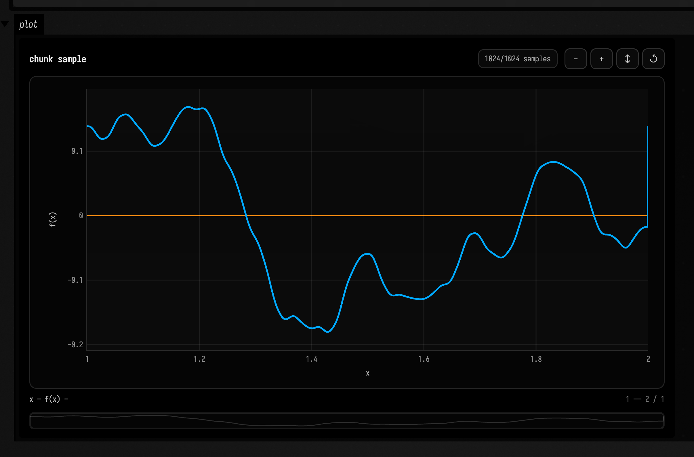
Functions.TimelineChunk.weightAt
Chunk weights report the local fade, gain, and window contribution at a time.
Simple
Returns the chunk's blend weight at the midpoint of its domain.
val w = Functions.TimelineChunk(sin(2.0), domain = 0.0..1.0).weightAt(0.5)Creative
:::static
with(Functions) {
    val ch = Functions.TimelineChunk(
        saw(0.2),
        domain = 0.0..1.0,
        window = spliceWindow(0.2, 0.2, 0.0..1.0),
        gain = valueNoise(1, 4.0, 0.2),
    )
    val w = ch.weightAt(0.6)
    val f = fn(name = "chunk weight") { x -> ch.weightAt(x) }
    f.plot()
}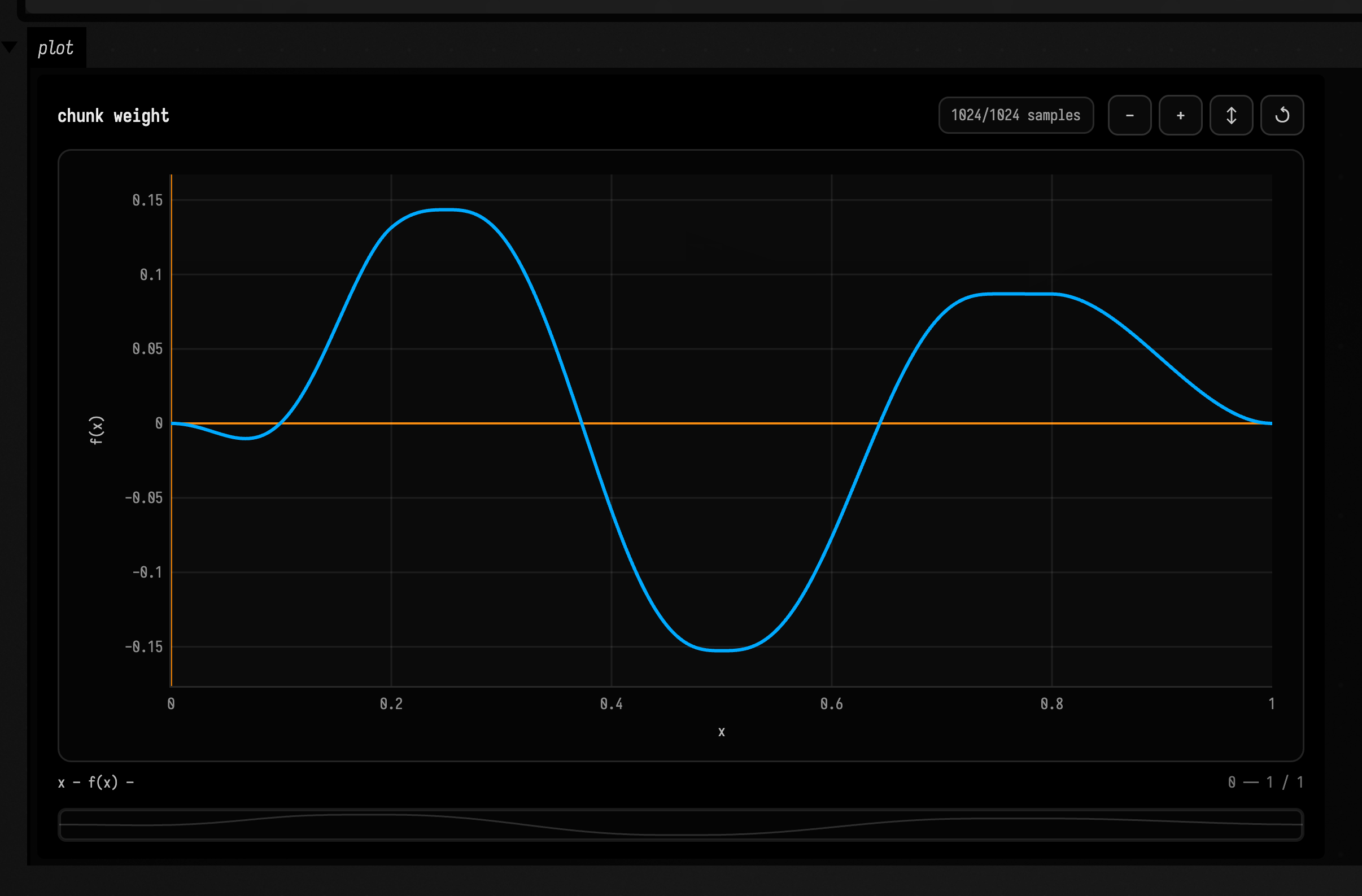
TimelineGraph.eval / invoke
Timeline graphs evaluate the active placed chunks at a given time.
Simple
Evaluates the timeline graph at x = 0.4.
val g = timelineGraph {
    sin(2.0).place()
}
val y = g.eval(0.4)
Creative
:::static
with(Functions) {
    val g = timelineGraph {
        pulseTrain(0.11).place(duration = 0.7)
        fbm(8, 3.0, 0.4).overlap(0.2, blend = ADD)
    }
    val y = g(0.9)
    g.asFn("graph eval").plot()
}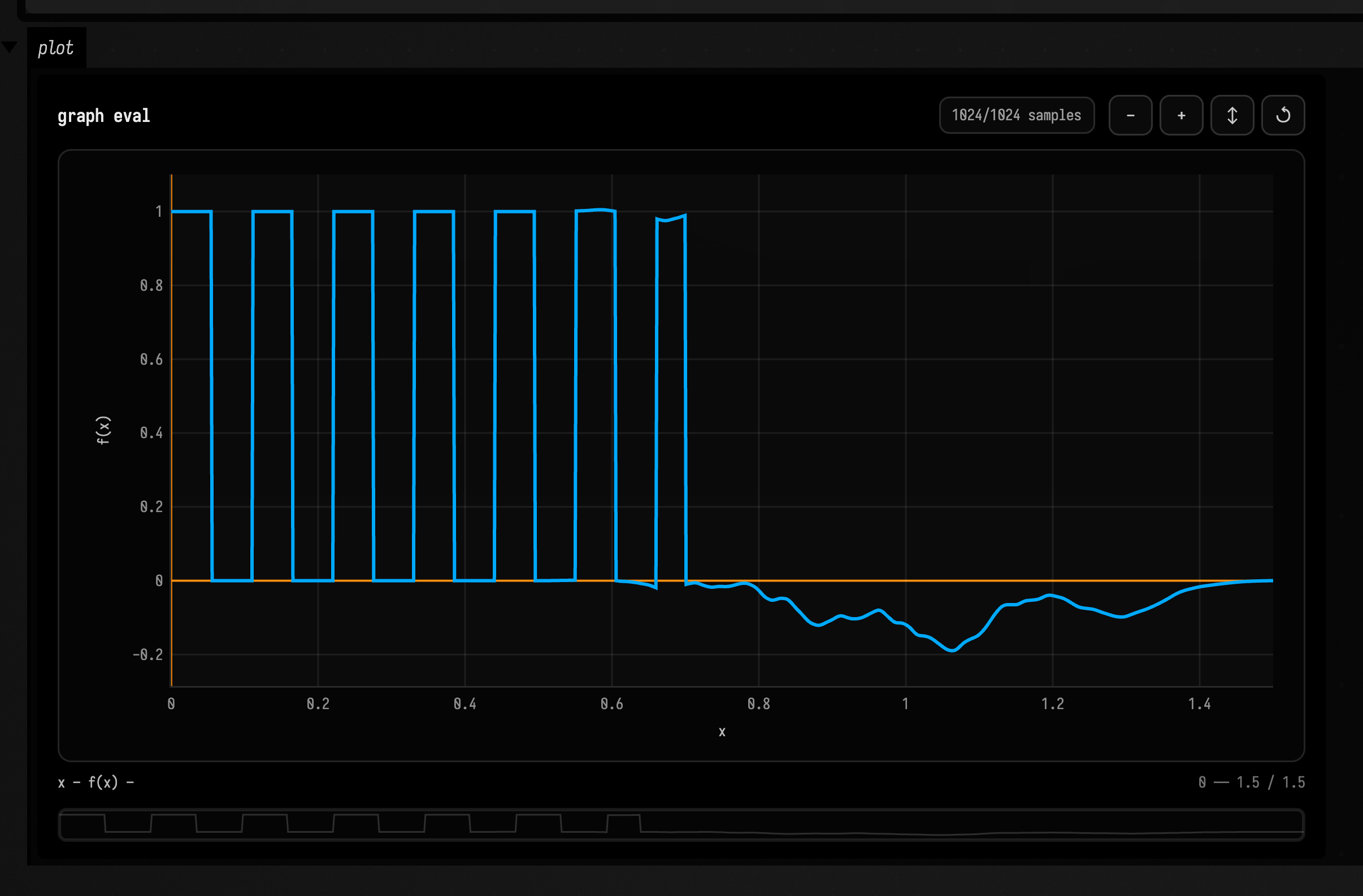
TimelineGraph.asFn / tap
Timeline graphs can be exposed as ordinary functions or sampled as delayed taps.
Simple
Exposes the timeline graph as a named Fn.
val f = timelineGraph {
    sin(2.0).place()
}
    .asFn("main")
Creative
:::static
with(Functions) {
    val delayed = timelineGraph {
        saw(0.2).place()
    }
        .tap(offset = 0.12, name = "echoTap")
    delayed.plot()
}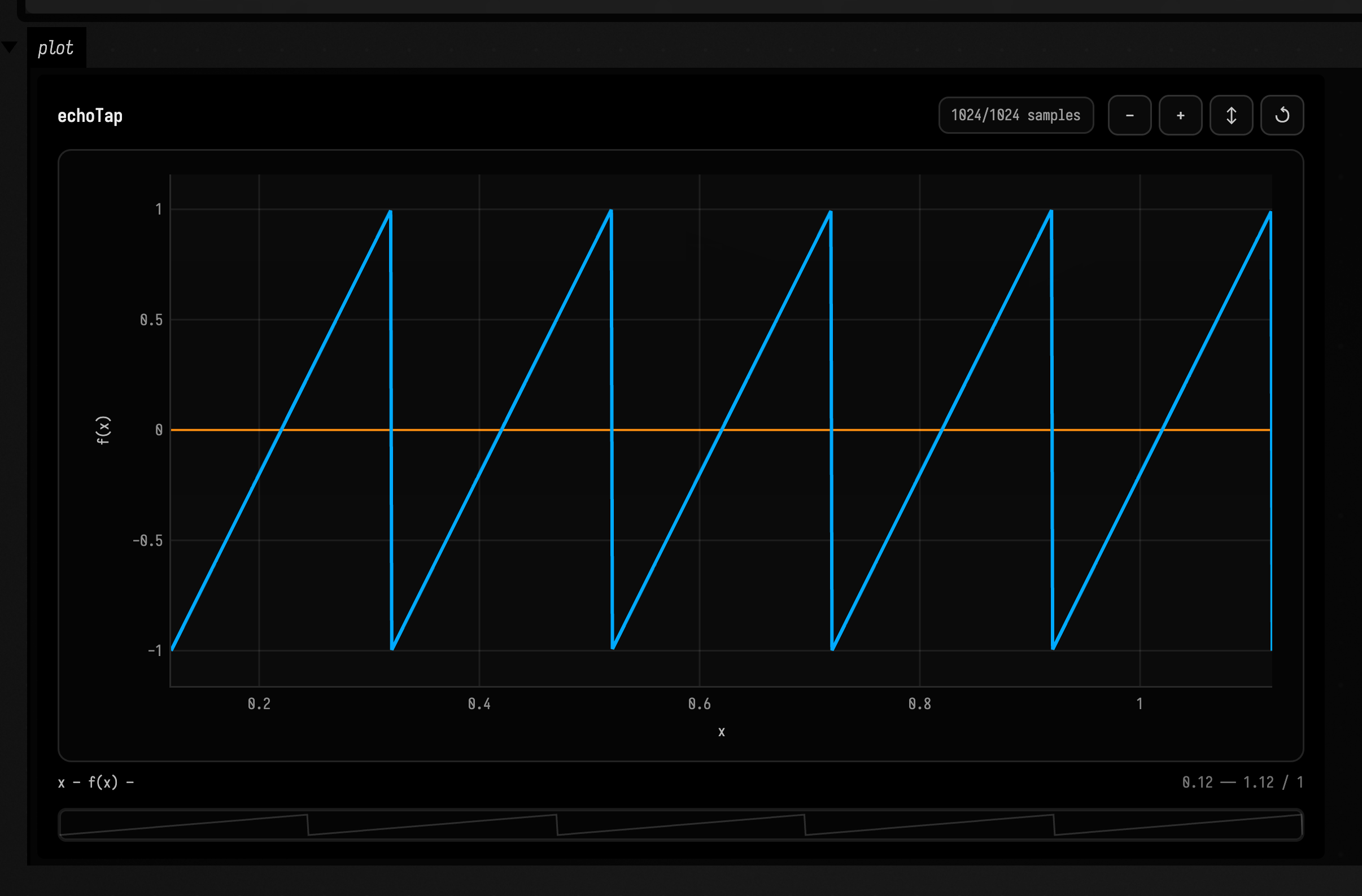
Functions.TimelineBuilder helpers
Builder helpers are the imperative timeline controls used by timeline { ... } and timelineGraph { ... }.
mark / marker
Timeline markers name positions so later placements can jump back to them.
Simple
Creates a timeline builder and records a mark named A at the current time.
val t = timeline {
    mark("A")
}
Creative
:::static
with(Functions) {
    val t = timeline {
        mark("intro", 0.5)
        moveToMark("intro", 0.2)
        sin(2.0).place()
    }
    t.plot()
}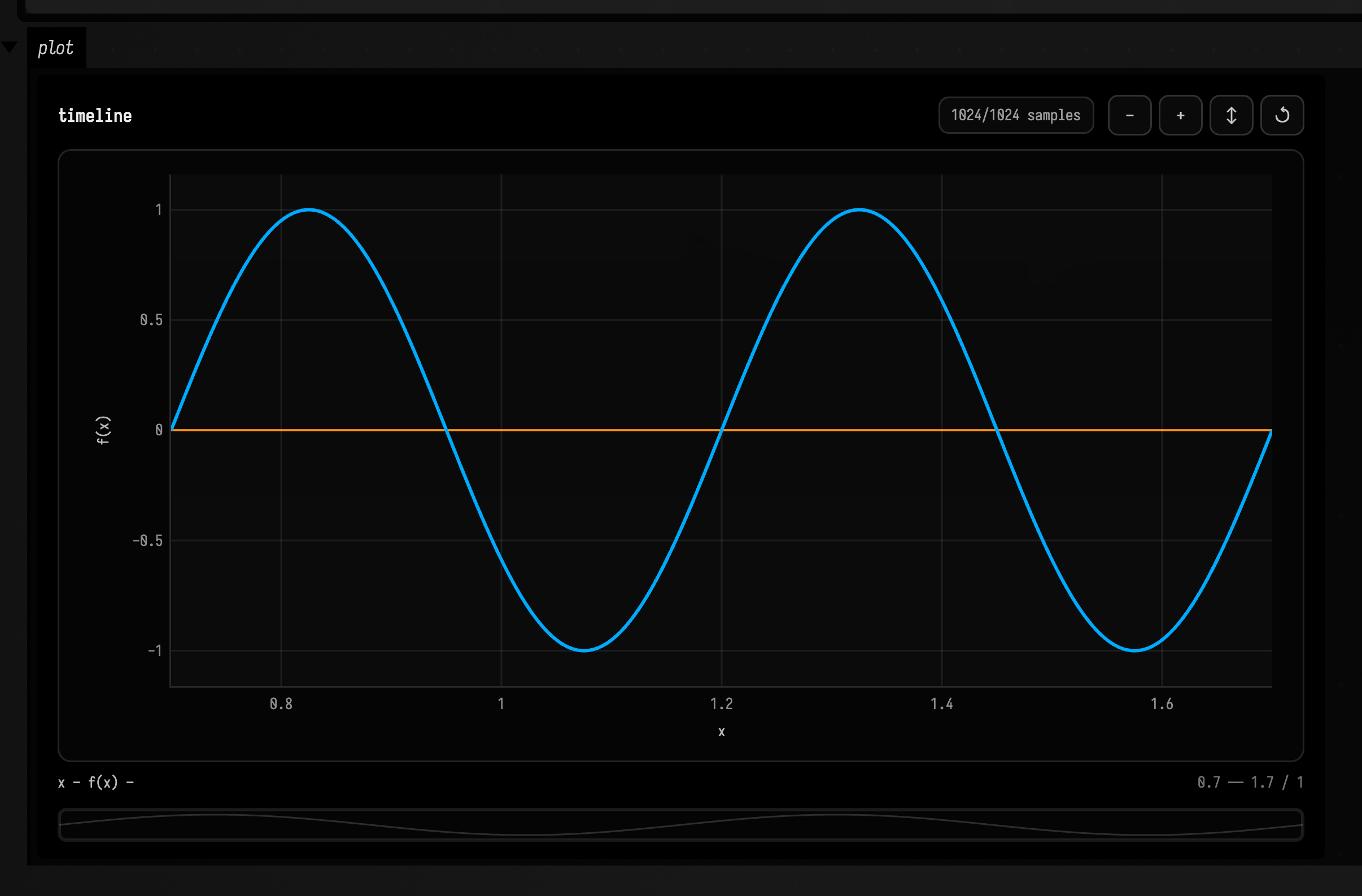
moveTo / moveToMark / advance / rewind
Timeline cursor controls place the next chunk at an absolute or relative time.
Simple
Moves the builder cursor to 0.3, advances it, then rewinds it slightly.
val t = timeline {
    moveTo(0.3)
    advance(0.2)
    rewind(0.1)
}
Creative
:::static
with(Functions) {
    val t = timeline {
        mark("drop")
        advance(0.4)
        moveToMark("drop", 0.15)
        pulseTrain(0.12).place()
    }
    t.plot()
}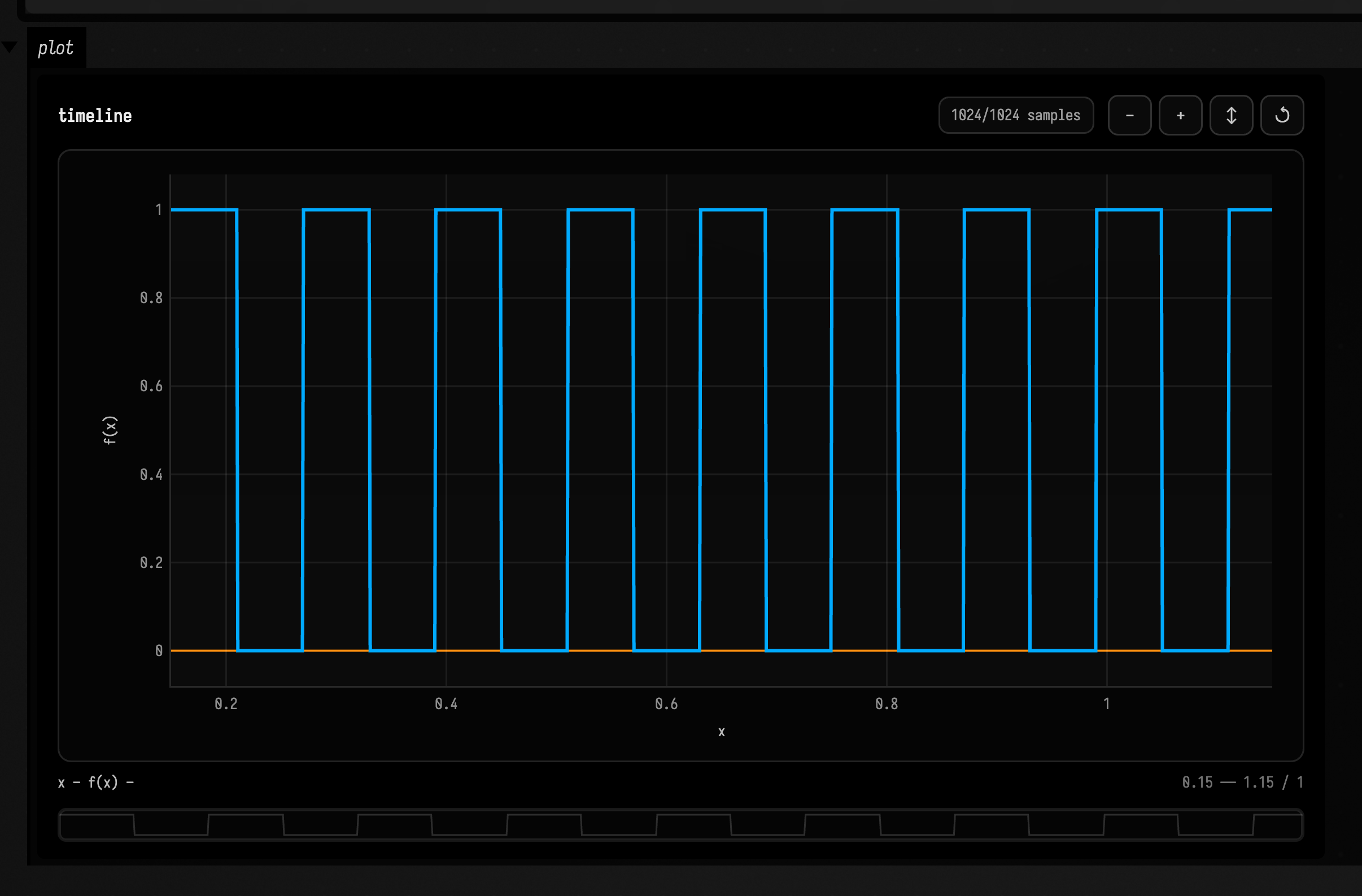
repeatToFit / stretchToFit
Fit helpers fill a target duration by wrapping or stretching a source.
Simple
Places repeated copies of the source function until two timeline units are filled.
val t = timeline {
    repeatToFit(sin(2.0), duration = 2.0)
}
Creative
:::static
with(Functions) {
    val t = timeline {
        stretchToFit(fbmPerlin(9, 2.0, 0.6), duration = 3.5, blend = ADD, gain = 0.45)
    }
    t.plot()
}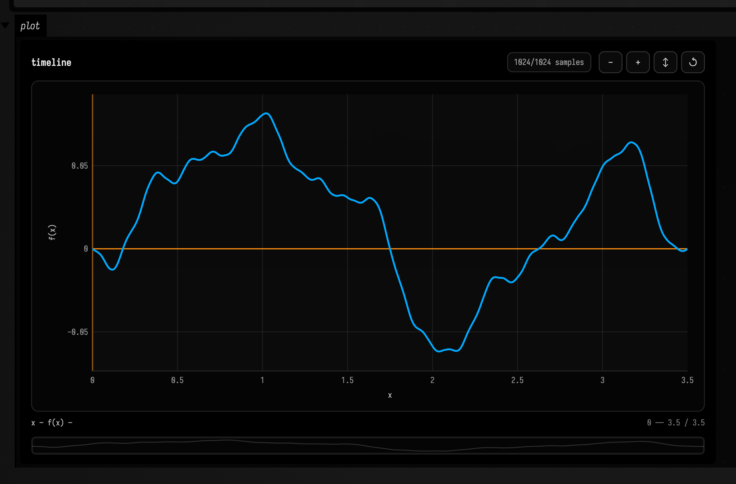
Fn.place / overlap / splice
Placement helpers add source functions to the active timeline with optional joins.
Simple
Places the sine function at the builder's current time.
val t = timeline {
    sin(2.0).place()
}
Creative
:::static
with(Functions) {
    val t = timeline {
        saw(0.18).place(duration = 1.1)
        pulseTrain(0.1).overlap(0.2, blend = ADD)
        fbm(4, 2.0, 0.2).splice(lookBack = 0.15, duration = 0.6)
    }
    t.plot()
}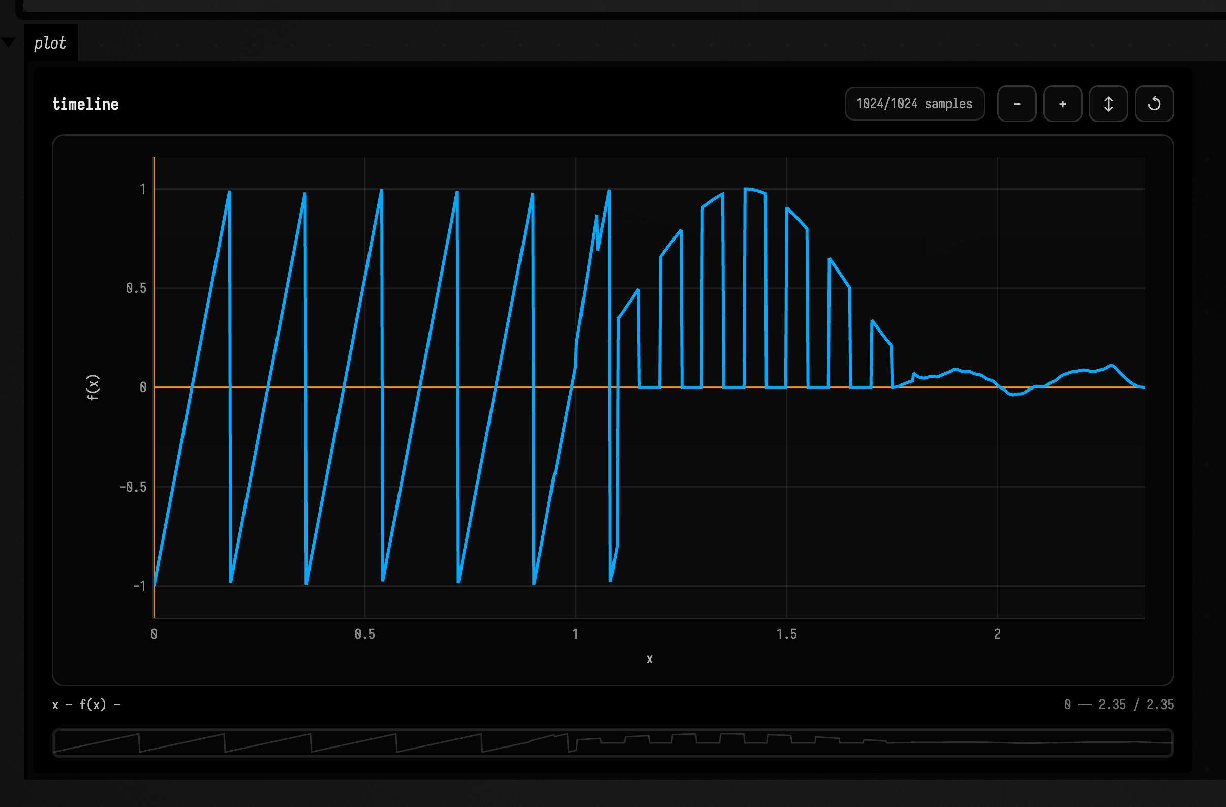
chunks / buildGraph / build
Builder outputs expose the placed chunks as graphs or ordinary functions.
Simple
Builds a graph from placed chunks and creates an empty named timeline.
val g = timelineGraph {
    one().place()
}
val cs = timeline(start = 0.0) {}.withName("empty")
Creative
:::static
with(Functions) {
    val f =
        Functions.TimelineBuilder(start = 0.0)
            .apply {
                sin(2.0).place()
                fbm(3, 4.0, 0.3).overlap(0.1, blend = ADD)
            }
            .build(name = "stacked")
    f.plot()
}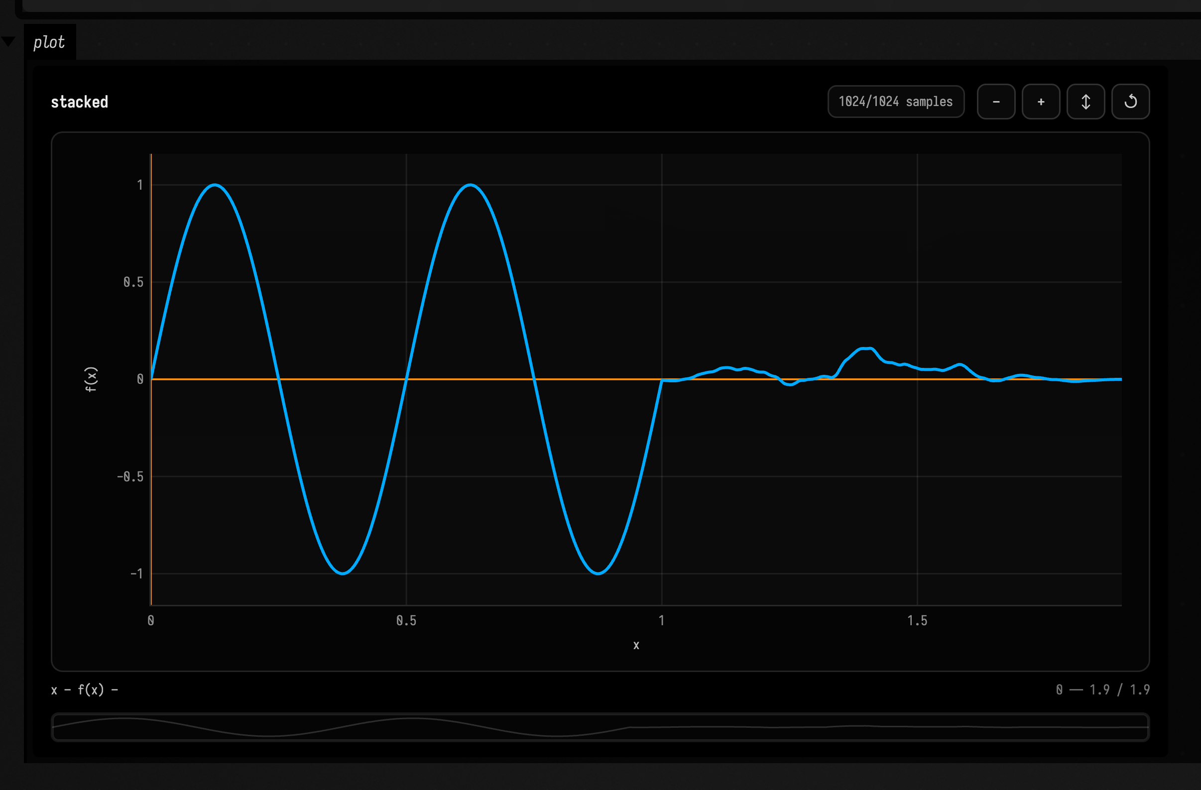
RBF kernels and interpolator
RBF entries cover the kernels and direct interpolator object behind the rbf(...) convenience functions.
RbfKernels.linear / quadratic / cubic / thinPlate
Built-in RBF kernels choose the shape used for radial fitting.
Simple
Interpolates the two points with a linear radial basis kernel.
val f = rbf(points(0.0 to 0.0, 1.0 to 1.0), kernel = RbfKernels.linear)Creative
:::static
with(Functions) {
    val f =
        rbf(points(0.0 to 0.0, 0.3 to 1.0, 0.8 to -0.5, 1.0 to 0.2), kernel = RbfKernels.thinPlate, smoothing = 1e-3)
    f.plot()
}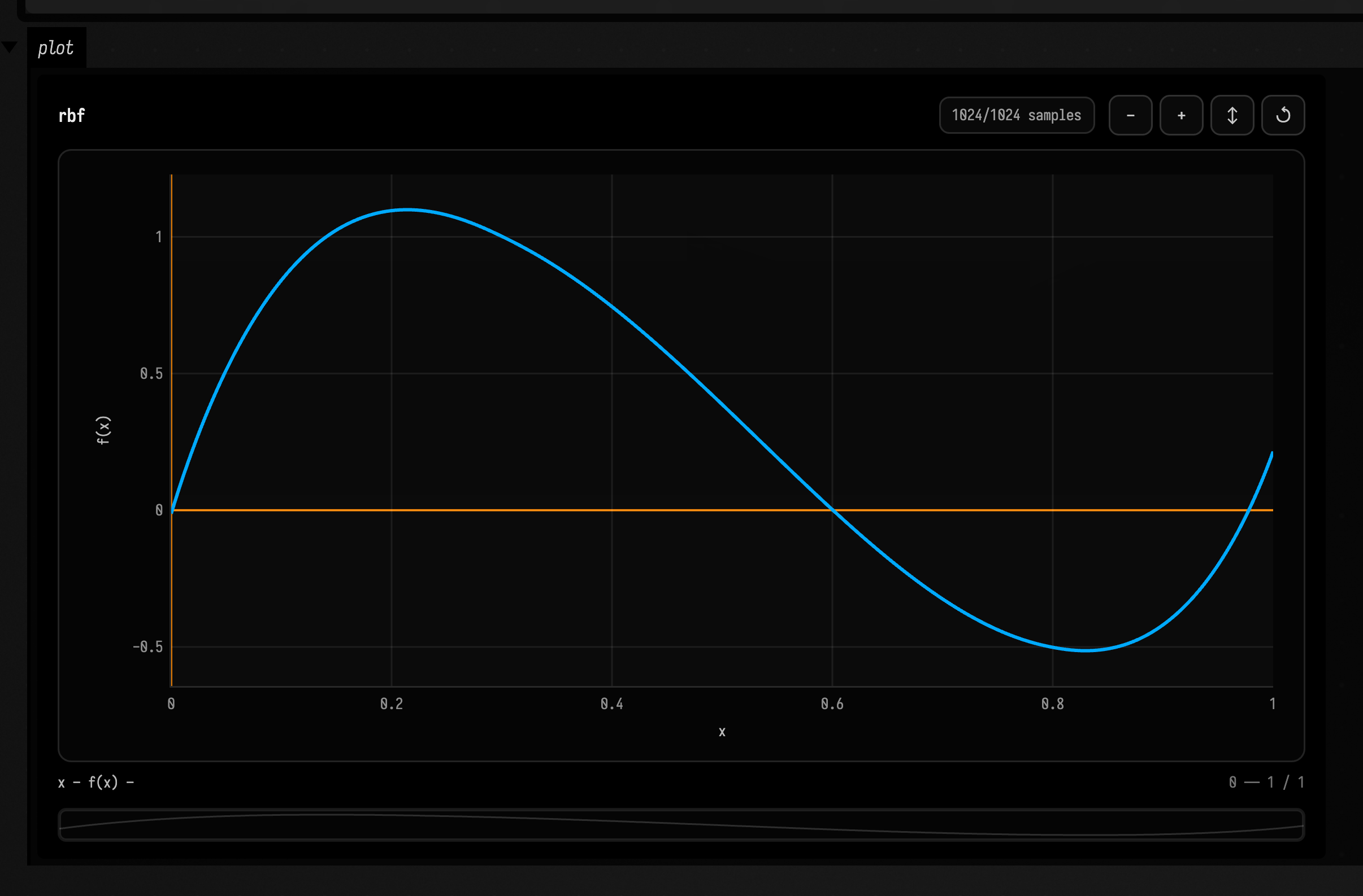
RbfKernels.gaussian / multiquadric / inverse*
Parameterized RBF kernels tune how strongly samples influence nearby x positions.
Simple
Interpolates the points with a Gaussian radial basis kernel.
val f = rbf(points(0.0 to 0.0, 1.0 to 0.4), kernel = RbfKernels.gaussian(2.0))Creative
:::static
with(Functions) {
    val f = rbf(points(0.0 to 0.2, 0.4 to 0.9, 1.0 to -0.1), kernel = RbfKernels.inverseQuadratic(0.5), base = sin(2.0))
    f.plot()
}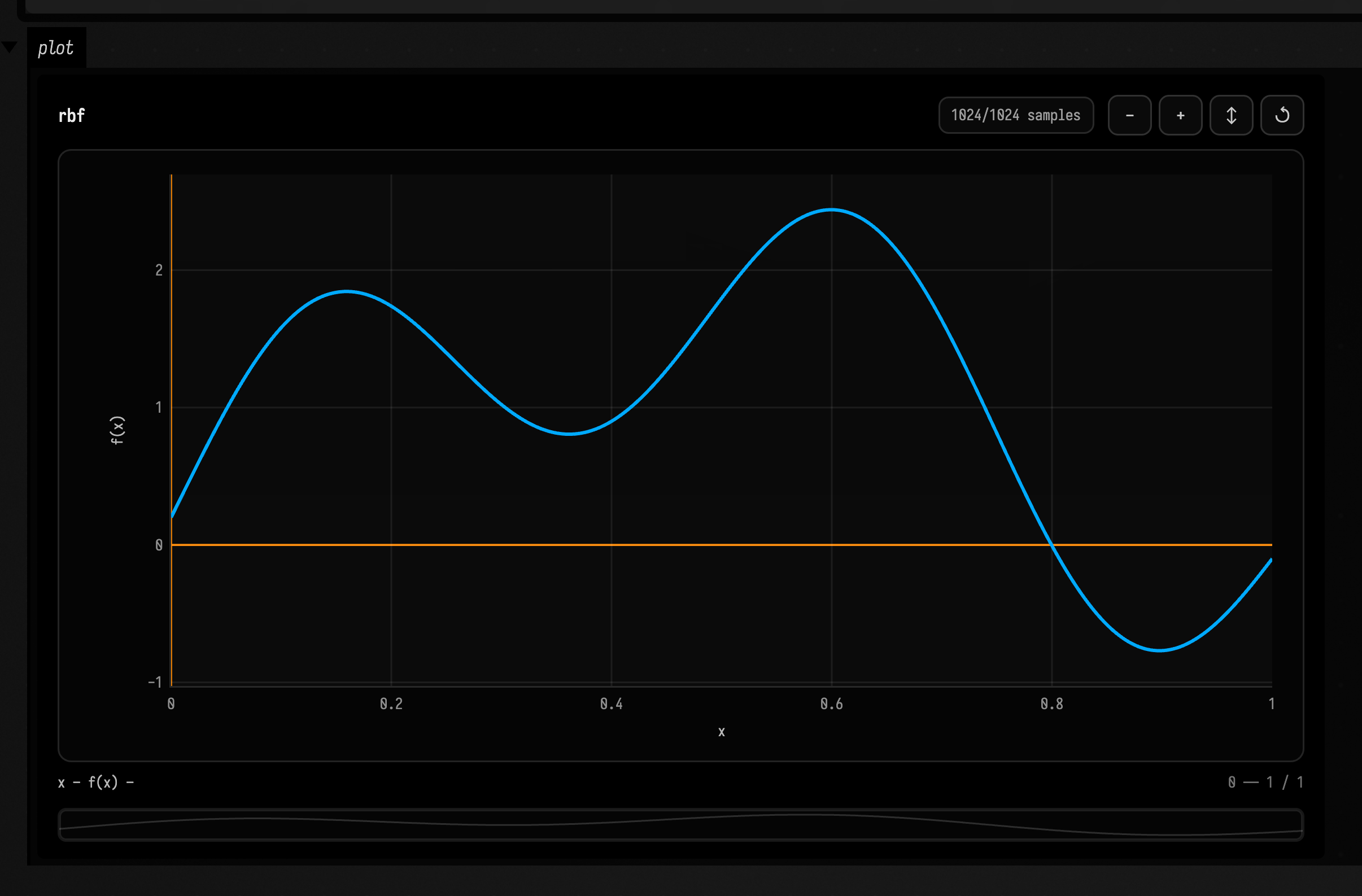
RbfInterpolator.eval
An RBF interpolator can be kept as an object and sampled directly.
Simple
Evaluates the cubic radial basis interpolator halfway between its two points.
val i = RbfInterpolator(points(0.0 to 0.0, 1.0 to 1.0), RbfKernels.cubic)
val y = i.eval(0.5)
Creative
:::static
with(Functions) {
    val i = RbfInterpolator(
        points(0.0 to 0.0, 0.2 to 0.9, 0.9 to -0.2),
        RbfKernels.gaussian(3.0),
        smoothing = 1e-4,
        base = sin(1.0),
    )
    val y = i.eval(0.63)
    val f = fn(name = "rbf interpolator") { x -> i.eval(x) }
    f.plot()
}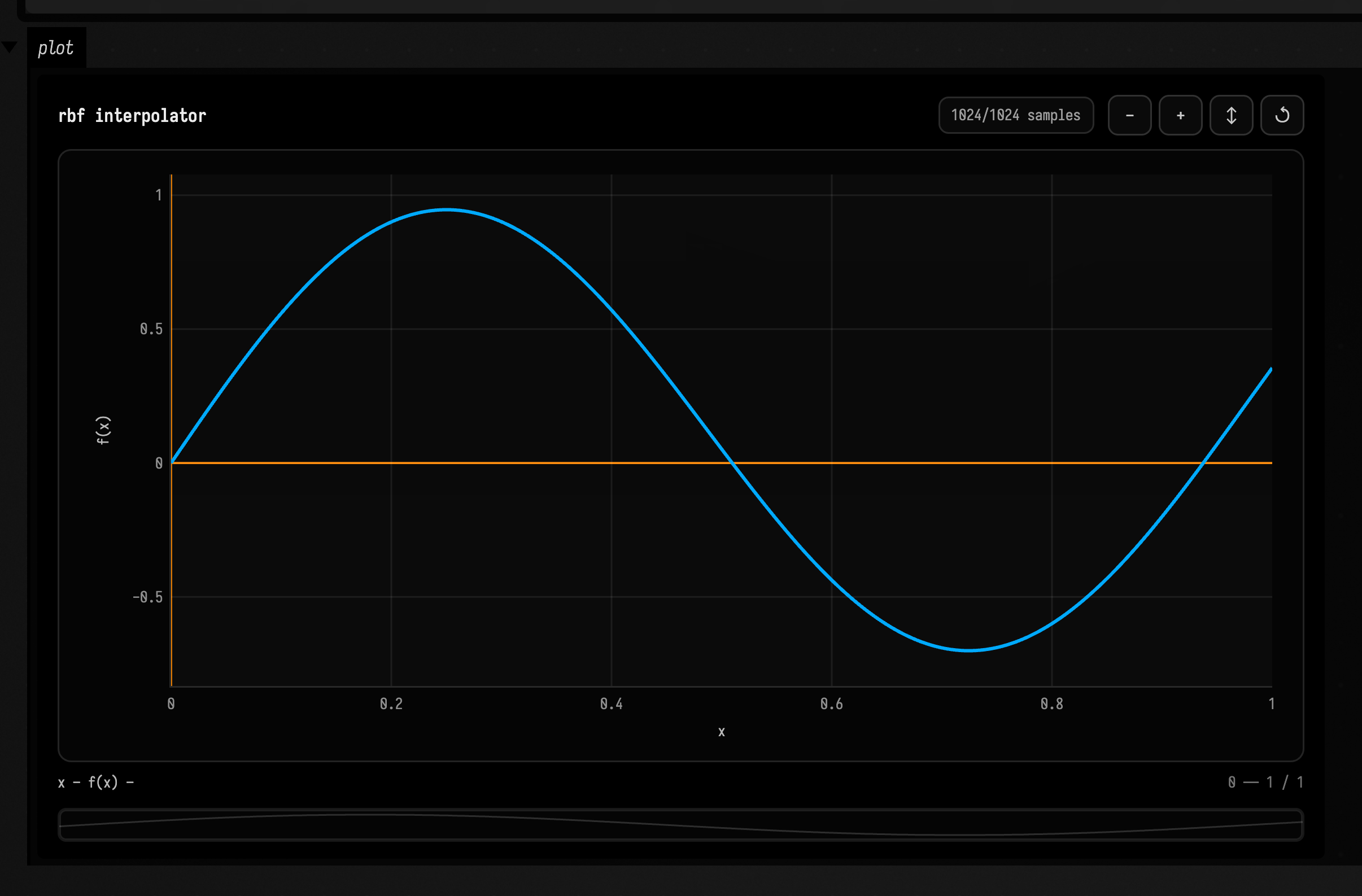
Browsing a function through its component graph
The final plot answers “what shape did I make?” browseGraph() answers “how did each occurrence become part of that shape?” It keeps the root function’s x-axis fixed while you select nodes in the structural graph:
:::static
with(Functions) {
    val gesture = (sin(2.0).shift(0.12) * tween(0.15, 1.0, 0.0..1.0, Functions.Easing.CUBIC_IN_OUT)).softClip(0.8)

    gesture.browseGraph(channel = "components")
}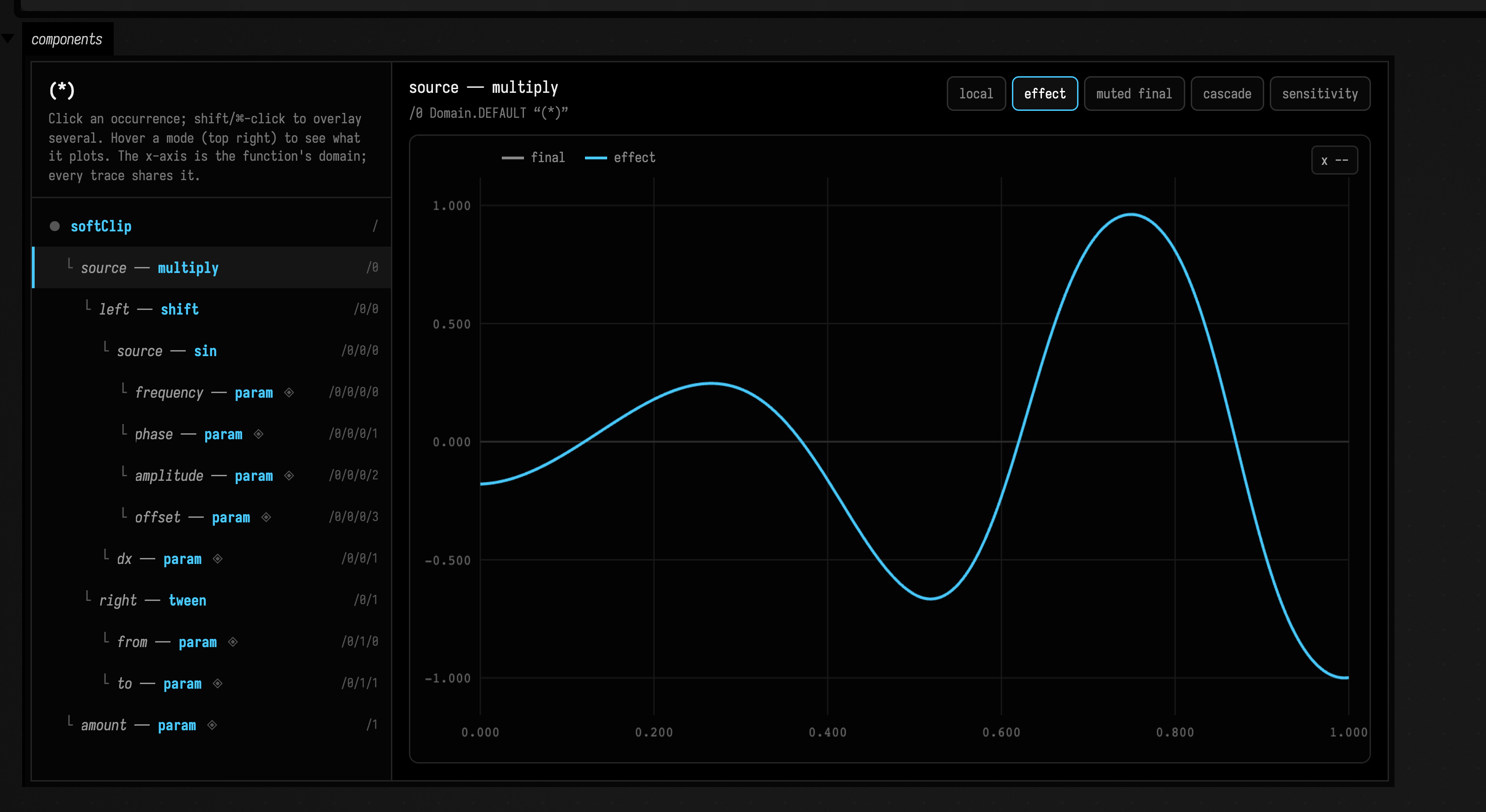
The browser always leaves the final curve visible in gray. The selected cyan trace has five views:
- local samples the selected subgraph directly on the final x-axis;
- effect replaces that exact occurrence with a neutral signal, rebuilds the root, and plots
final - muted; - muted final shows the rebuilt root without that occurrence;
- cascade steps the selected component up its ancestor chain one transform at a time, so you watch a raw piece become the final shape — a slider walks leaf → root, every stage on the shared x-axis;
- sensitivity sweeps the selected numeric node across a range and overlays the resulting family of final curves, so you can see how much that one number moves the finished gesture.
Shift- or ctrl/command-click nodes in the sidebar to overlay several occurrences at once for side-by-side comparison.
Local and effect diverge in the cases you care about. A sine below shift, warp, repeat, multiplication, or a timeline may look ordinary locally while its effect shows where it actually lands in the finished gesture. Every graph occurrence has its own path, so a shared function used in two places can be inspected twice in context.
val trace = gesture.graphTrace(samples = 256)
val shiftedSine = trace.nodes.first { it.op == "sin" }

println(shiftedSine.path)
println(shiftedSine.local.take(4))
println(shiftedSine.effect.take(4))
graphTrace(...) is the non-HTML form for tests, analysis, and agents. It returns the shared x coordinates, final samples, and local/muted/effect arrays for each occurrence, plus the numeric-node value sweeps behind the sensitivity view (pass sensitivitySteps to control the sweep resolution). maxDepth and maxNodes bound the work for unusually large generated graphs.
Effect is called contextual effect rather than contribution. For addition it behaves like an additive decomposition; for clipping, division, modulation, and other nonlinear parents it answers a stricter counterfactual question: “what changes in the final output if this occurrence is neutralized?”
Watching a rewrite happen
The occurrence browser answers "how did each piece become the final shape?"; browseRewrite(...) answers "what did each rewrite do to that shape?" It applies the rules one at a time and steps through the result on the same time-base, drawing before (dashed), after (cyan), and delta (orange) for each rule:
:::static
with(Functions) {
    val gesture = (sin(2.0).shift(0.12) * tween(0.15, 1.0, 0.0..1.0, Functions.Easing.CUBIC_IN_OUT)).softClip(0.8)

    gesture.browseRewrite(
        """
#fnrewrite
sin => op=triangle
**/[role=amplitude] => *= 0.5
""",
        channel = "rewrite",
    )
}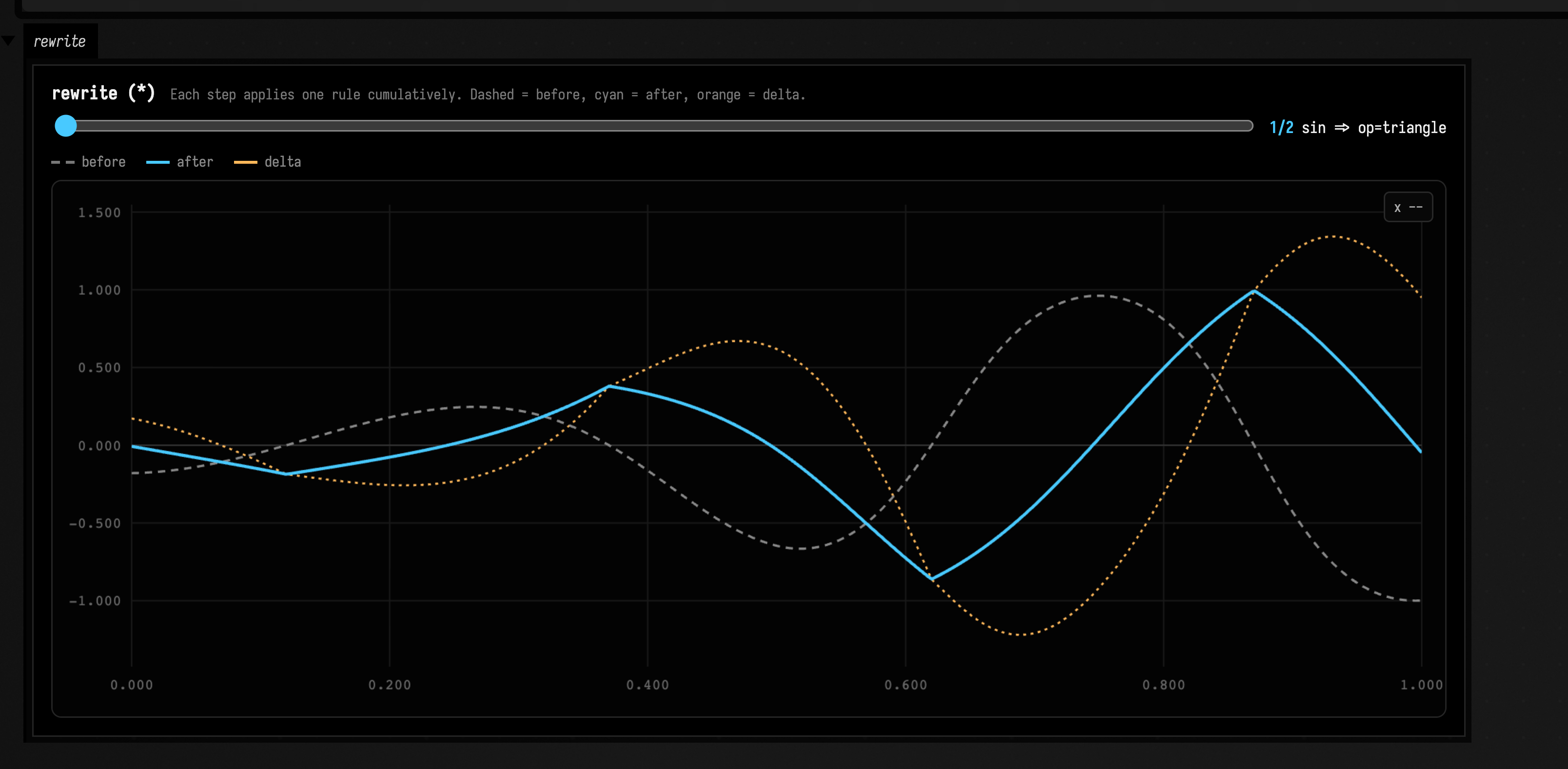
graphRewriteTrace(...) is the non-HTML form, and it also accepts a List<FnGraphRule>, so the same before/after lanes work for the pattern rules and programmatic rules described below, not just the string DSL. Together, the two browsers close the loop between structural editing and perceptual confirmation: rewrite the graph, then watch exactly which occurrence moved and by how much.
Fn graph inspection and rewrite language
Fn values carry a best-effort structural graph alongside their evaluator. Ordinary sampling still uses the evaluator; the graph is there so a function can be inspected, deep-copied, visualized, and rewritten without reverse-engineering a Kotlin closure. Constructors and combiners in the standard family attach graph nodes with operation names, child edges, numeric metadata, and rebuild recipes. Opaque fn { ... } functions still evaluate normally, but rewrite passes cannot see inside their lambda bodies.
The rewrite language is a compact "selector => action" layer over Fn.rewriteGraph(...). It is closer to XPath/CSS/glob selectors than to JSON tools: the thing being matched is a labeled occurrence path through a function graph.
Simple
Inspects the graph of a nested function, then rewrites the saw under a sin into a triangle.
val base = sin(sin(saw(0.25)))
val changed =
    base.rewriteKotlin(
        """
#fnrewrite
sin/*/saw => op=triangle
""",
    )
Creative
:::static
with(Functions) {
    val base = sin(sin(saw(0.25))).withName("nested carrier")
    val changed =
        base.rewriteKotlin(
            """
#fnrewrite
sin/*/saw => op=triangle
sin/**/[tag=number][value>0.2] => = 0.5
""",
        )

    :::fold render the before/after graphs
    // The two graphs are stacked, not side by side — the original grid was a single column.
    markdown(
        "graph",
        """
        #### before
        ${base.graphSvg(width = 1060, nodeWidth = 186.0, nodeHeight = 52.0, xGap = 200.0, yGap = 70.0, maxDepth = 5)}

        #### after
        ${changed.graphSvg(width = 1060, nodeWidth = 186.0, nodeHeight = 52.0, xGap = 200.0, yGap = 70.0, maxDepth = 5)}
    """,
        width = 1120,
    )
    :::endfold
}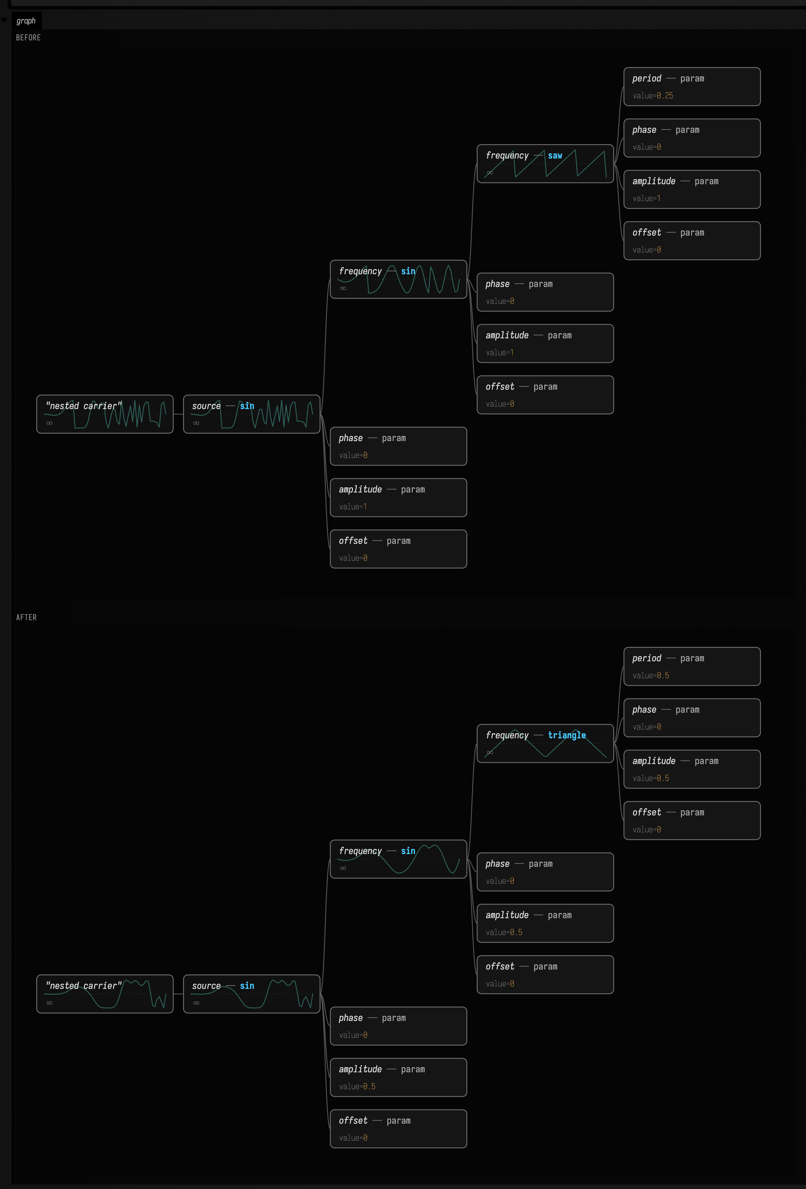
The first rule matches a saw occurrence whose parent is any node and whose grandparent is sin. The second rule finds numeric nodes anywhere under a sin and changes values greater than 0.2 to 0.5. The graph view is a better first read than text here: the operation swap and constant rewrites become visible as topology and labels.
Each non-constant card also carries a sparkline: a faint teal waveform drawn behind the labels that samples the sub-expression rooted at that node (the operator together with all of its parameters) across its own domain, falling back to the unit interval when the domain is unbounded. A dashed baseline marks zero whenever the signal crosses it. Constants are left blank because a flat line has no shape to plot. So the topology tells you what changed, and the sparkline at each node shows how the shape at that point changed as a result. Pass sparklines = false to graphSvg(...) to suppress the waveforms and get bare cards.
The interactive loop: compile, preview, commit
rewrite(...) is forgiving; a sketch or a performance needs it to be. For deliberate editing, especially from an agent, use the three-stage API:
val source = (saw(0.2) * 0.5).withName("gesture")
val spec =
    """
#fnrewrite
saw -> op=triangle                 # `->` reads naturally
**/[role=amplitude] → *= 0.75      # unicode arrows are welcome too
parent=notHere => drop             # useful experiment; currently unmatched
"""

val program = compileFnRewrite(spec)
println(program.diagnosticText())

val preview = source.previewRewrite(spec)
println(preview.summary())

val committed = source.rewriteChecked(spec)
compileFnRewrite(...) never needs a function graph. It checks the language, retains valid rules, and returns line-addressed errors and warnings. previewRewrite(...) applies those rules to an immutable copy and records every matched path, role, before/after operation, no-op, and unmatched rule. rewriteChecked(...) refuses a program with errors, where ordinary rewrite(...) presses on.
When the rules contain Kotlin @{...} expressions, use previewRewriteKotlin(...) and rewriteKotlinChecked(...). They compile expressions in the current Field box just like rewriteKotlin(...), so preview and commit see the same live variables, imports, and helper functions.
That gives humans a pleasant rhythm (write, inspect, listen or look, commit) and gives agents a bounded evidence loop:
- Compile and fix every error.
- Preview and read
summary(). - Treat unmatched rules and matched/no-op applications as hypotheses to reconsider, not silent success.
- Plot or sample the previewed function when structural success also needs perceptual confirmation.
- Commit with
rewriteChecked(...)once the report matches the intention.
The summary is compact and deterministic enough to paste into chat or a transcript. A typical report starts with FnRewrite: 3 rule(s), 2 match(es), 2 change(s), then lists unmatched selectors, diagnostics, and paths such as #1 path=/0 op=saw changed -> triangle.
Rewrite rule shape
A rewrite spec is a sequence of rules. Rules can be separated by newlines or semicolons. A rule has one selector on the left and one or more actions on the right:
selector => action
selector => action, action
selector => action | action
Commas and pipes on the RHS both mean "then". Actions are applied left-to-right to the copied node. This matters for numeric edits:
**/[value>0.2] => *= 2.0, += 1.0That rule doubles the current numeric value, then adds one to the doubled value.
Lines starting with # or // are comments. The #fnrewrite header is optional for runtime parsing, but useful inside Kotlin triple-quoted strings because the Monaco language extension recognizes it:
val spec =
    """
#fnrewrite
sin/**/[tag=number] => *= @{1.0 + depth * 0.1}
"""
Inline comments are supported too, including after actions. The canonical arrow is =>; ASCII -> and Unicode → are exact aliases. Monaco highlights, diagnoses, and completes both embedded #fnrewrite strings and standalone fnrewrite models.
Selector basics
A selector is a set of terms. Whitespace and & both mean "and":
saw
role=frequency
parent=sin role=amplitude
parent=sin & role=amplitude
tag=number
The older terse selector style is still supported:
sin.frequencyThat reads as "a node connected through the frequency role on or under a sin-ish occurrence". Prefer path selectors for new code when ancestry matters; they are more explicit.
Useful term forms:
| Term | Matches |
|---|---|
sin |
Matches an operation, incoming role or tag named sin. Use op=sin when only the operation should count. |
number |
Matches a node tagged as numeric metadata. Numeric actions apply only when it also has a value entry. |
const / param / opaque |
Matches common node classes by their tags. Constants and parameters normally expose numeric metadata; an opaque node hides its internal construction. |
op=saw |
Matches the current node’s operation exactly. It does not select an incoming parameter merely named saw. |
role=frequency |
Matches a node reached through a frequency parameter edge. This selects the use of a node within its parent. |
edge=frequency |
Selects the incoming frequency edge. edge is an alias for role. |
parameter=frequency |
Selects the same edge as role=frequency. Use whichever spelling makes the rule easier to read. |
parent=sin |
Matches when the immediate parent operation is sin. |
under=sin |
Matches anywhere below a sin, at any depth. |
name=lead |
Matches the function’s public name. Give a function a name when it needs a stable target independent of its operation. |
tag=number |
Requires membership in the node’s tag set. This avoids the broader operation-or-role interpretation of a bare term. |
depth=2 |
Matches occurrences two edges below the root. The root is depth zero. |
Path selectors
Path selectors are slash-separated occurrence matches:
sin/saw
sin/*/saw
sin/**/saw
/multiply/**/[tag=number]
The matched node is always the current node being considered for rewrite. An unanchored path can match any suffix of the current root-to-node occurrence path. A leading / anchors the match at the graph root.
| Example | What it matches |
|---|---|
sin/saw |
Matches a saw occurrence directly below a sin occurrence. An unanchored path can match a suffix of the root-to-node path. |
sin/*/saw |
Matches a saw with exactly one intermediate node below sin. * consumes one node in the path. |
sin/**/saw |
Matches a saw at any depth below sin, including an immediate child. ** consumes zero or more intermediate nodes. |
/multiply/**/saw |
Requires multiply at the graph root, then finds descendant saw occurrences. The leading slash prevents a match from starting deeper in the graph. |
**/[tag=number][value>0.2] |
Filters the current path segment by both predicates. Here it selects numeric-tagged nodes whose value exceeds 0.2. |
Examples:
sin/*/sawMatches saw nodes that are children of children of a sin.
sin/**/sawMatches saw nodes at any depth below a sin, including direct children.
/multiply/**/[tag=number]Matches numeric nodes anywhere under a root multiply graph.
Because graph nodes may be shared, the match is occurrence-based. The same Fn object can appear through multiple paths. Whether those paths collapse to one copied node depends on preserveSharing; by default rewriteKotlin(...) copies by occurrence so path-sensitive edits are unsurprising.
Predicates
Predicates live inside path segments:
**/[op=const]
**/[role=frequency]
**/[tag=number][value>0.2]
**/[depth>=2][index=0]
Supported predicate keys:
| Predicate example | Value being tested |
|---|---|
**/[op=const] |
Tests the graph operation name. This selects constant operations wherever they occur. |
**/[role=frequency] |
Tests the incoming edge role; edge, param and parameter are aliases. The root has no incoming edge. |
**/[tag=number] |
Tests membership in the graph tag set. Tags describe capabilities or categories beyond the operation name. |
**/[name=lead] |
Tests the function’s public name. Unnamed nodes do not match a named target. |
**/[depth>=2] |
Tests the number of edges from the root. Here only grandchildren and deeper occurrences match. |
**/[index=0] |
Tests the child’s index within its parent. Zero selects the first child occurrence. |
**/[value>0.2] |
Tests the node’s numeric value metadata. Numeric comparisons apply when both operands parse as numbers. |
**/[seed=7] |
Other keys look in the node’s numeric, string, boolean or long metadata maps. Use only a key carried by the selected operation; an unknown key may simply match nothing. |
Supported comparisons are =, !=, >, <, >=, and <=. Numeric comparisons are used when both sides can be parsed as numbers; otherwise equality is case-insensitive string equality.
Actions
Actions rebuild or relabel the matched copied node:
| Action | Effect |
|---|---|
drop, prune, zero |
Replaces the matched node with a zero function on the copied node’s domain. All three spellings have the same effect. |
op=sin |
Rebuilds the node as a sine operation using available role-addressed children and metadata. An impossible reconstruction is left unchanged and reported by preview. |
replace=triangle |
Rebuilds the node as a triangle operation. This is an alias for op=triangle. |
name=lead |
Sets the copied function’s public name. Later selectors can target it with name=lead. |
domain=all |
Sets the copied node’s domain to Domain.ALL. This changes domain metadata rather than sampling new values. |
domain=default |
Sets the copied node’s domain to Domain.DEFAULT. Use it to restore the standard domain label. |
domain=0.0..1.0 |
Sets an explicit domain interval on the copied function. The interval belongs to this matched node. |
= 0.5 |
Replaces the node’s numeric value with 0.5. Nodes without numeric value metadata are unchanged. |
*= 2.0 |
Doubles the current numeric value. Actions run left to right, so a following addition sees the doubled value. |
/= 2.0 |
Halves the current numeric value. It affects the matched numeric parameter rather than scaling the entire output graph. |
+= 0.1 |
Adds 0.1 to the current numeric value. Use a role selector to target a particular parameter. |
-= 0.1 |
Subtracts 0.1 from the current numeric value. A nonnumeric match is reported as a no-op rather than failing the whole rewrite. |
Numeric actions apply only to nodes with a numbers["value"] metadata entry. That usually means constants and parameter nodes. If a numeric action lands on a non-numeric node, it is ignored rather than failing the whole rewrite.
op=... transmutes a node to another operation, reusing role-addressed children and scalar metadata. OpRegistry holds the whole vocabulary, and holds it once: the DSL validator and the Monaco editor consult the same object. Every target is one OpSpec, and they fall into three groups that rebuild differently:
- Generators — oscillators (
sin,cos,saw,triangle,square),pulseTrain, noise (whiteNoise,valueNoise,perlinNoise,fbm,fbmPerlin,randomWalk), windows (hannWindow,hammingWindow,blackmanWindow,gaussianWindow),gaussian,ramp,remap,step,smoothstep,tween,ease. These rebuild from whatever roles the source carries and fall back to factory defaults for the rest. Role names bridge across families, sosin => op=sawcarriesfrequencyover asperiod(via reciprocal) rather than resetting it. - Algebra —
add,subtract,multiply,divide, rebuilt from theleft/rightchildren. - Value transforms —
shift,scaleX,scaleY,offsetY,pow,exp,log,abs,sign,floor,flip,clamp,clip,softClip,fold,chebyshev,rectify,quantize,crush,wrapY, and the trig group (atan,atan2,hypot). These need an existingsourcechild, soclamp => op=softClipworks whilesin => op=clampis reported as a no-op (nothing to wrap) rather than silently doing something else.
Transmutation reports impossibility rather than guessing at it: if a target cannot be built from the matched node it is left unchanged and reported as matched/no-op in previewRewrite(...). Data-carrying ops such as piecewise, timeline, and rbf are known to selectors and validation but are not transmutation targets, because their identity lives in baked point/item data a foreign node cannot supply.
Kotlin on the RHS
Use @{ ... } for Kotlin expressions in numeric actions. The code inside is compiled in the current live Field box context by rewriteKotlin(...), and it receives a FnRewriteNumberContext as implicit receiver:
**/[tag=number] => *= @{1.0 + depth * 0.1}
**/[role=amplitude] => = @{if (parentOp == "sin") value * 0.5 else value}
Available names inside @{...}:
| Name | Meaning |
|---|---|
value |
current under the name a snippet actually writes, as in *= @{value * 1.1}. |
it |
current again, so a snippet can read like a lambda: = @{it * 2}. A plain property, not a real lambda parameter — nothing is shadowing it, and it inside a nested lambda wins as usual. |
op |
The op name of the matched node, from OpRegistry's vocabulary. |
role |
The role of the edge this node was reached by ("frequency", "amplitude", …), or null at the root. |
parameter |
Alias for role, for rules that read better as "which parameter am I". |
parentOp |
The immediate parent's op, or null at the root — "am I inside an fbm?" in one property. |
depth |
How many edges below the root this occurrence sits; the root itself is 0. |
path |
Child indices from the root down to this node — the same path a preview reports. |
ancestors |
The path elements from the root down to this node's parent, root first. Empty at the root. |
occurrence |
ancestors plus this node — the whole root-to-here path, which is what a path selector matches against. Rebuilt on every read, so bind it to a local rather than indexing it repeatedly. |
name |
The matched function's own name, if it was given one. Null for the great majority of nodes. |
domain |
The matched function's own domain, which can be narrower than the root's. |
numbers |
This node's numeric metadata — its own parameters, keyed by name. A constant carries value. |
strings |
This node's string metadata, for the ops that carry names or modes rather than numbers. |
booleans |
This node's boolean metadata — flags such as a wrap or clamp mode. |
longs |
This node's long metadata, typically seeds and counts. |
Kotlin RHS snippets can be multi-line. The last expression is returned:
**/[tag=number] => = @{
    val bias = if (role == "frequency") 1.25 else 1.0
    value * bias + depth * 0.05
}
The older ${...} form is still accepted for compatibility, but @{...} is the intended syntax because it can be written directly inside Kotlin raw strings without escaping.
rewrite versus rewriteKotlin
Use rewriteKotlin(...) in live Field code. It accepts all rewrite syntax, including @{...} RHS snippets:
val g =
    f.rewriteKotlin(
        """
#fnrewrite
sin/**/[tag=number] => *= @{1.1}
""",
    )
The lower-level rewrite(...) function is useful when the RHS is plain numbers and actions, or when you are supplying your own evaluator through FnRewriteOptions. It does not depend on the live-code compiler at all.
Programmatic rules, traces, and fixed points
The string language is the concise live-coding surface. The middle layer for larger experiments is FnGraphRule: a named predicate plus a replacement function. It uses the same bottom-up graph copier as rewrite(...), but returns a trace rather than only a new function.
val eliminateAddZero = FnGraphRule(
    name = "x + 0 -> x",
    matches = { c ->
        c.op == "add" && c.node.child("right")?.graphNode()?.numbers?.get("value") == 0.0
    },
    replace = { _, copy -> copy.graphNode().child("left") ?: copy },
)

val run = ((sin(2.0) + 0.0) + 0.0).rewriteUntilStable(eliminateAddZero)
val optimized = run.function
println("${run.stop}: ${run.events.size} edits in ${run.passes} passes")
This API is small, but it establishes the pieces needed for a more ambitious optimizer or evolving-function system:
graphMatches { ... }returns occurrence-sensitive matches with roles, ancestry, depth, and paths.firstGraphMatch { ... }is the short-circuit query form.graphMetrics { node -> cost }reports unique nodes, path occurrences, edges, depth, opacity, rebuildability, and a caller-defined cost.graphSignature()gives a deterministic structural signature without sampling or comparing evaluator closures.rewriteWithRules(...)performs one named, traced pass.rewriteUntilStable(...)performs bounded passes and stops withSTABLE,CYCLE, orMAX_PASSES.
Rules default to FIRST_MATCH at each node, which makes priority explicit. Use FnGraphRuleMode.ALL_MATCHES when several rules should chain on the same copied node. A bounded run is important in live art code: an oscillating rewrite should report a cycle, not disappear into the animation loop.
graphMetrics separates shared DAG nodes from path occurrences. Count unique nodes and a repeated motif disappears into one entry; count occurrences and it shows up as many. That is also the hook a cost-guided search needs: execution cost might charge each unique node, while visual or semantic complexity might charge each occurrence.
Pattern → template rewriting
The selector DSL edits one matched node in place. Its algebraic sibling is pattern => template, where both sides are graph shapes with metavariables. This is the term-rewriting surface a rewriting or evolving-function system reasons with. A metavariable ?x binds a whole subtree (and, if repeated, must bind structurally equal subtrees); a bare number matches a numeric node; a bare op matches by op; op(child, …) also constrains the leading children.
val simplified = ((sin(2.0) + 0.0) + 0.0).rewritePatterns(
    "add(?x, 0) => ?x", // additive identity, applied to a fixed point
    "multiply(?x, 1) => ?x", // multiplicative identity
)
println(simplified.function.graphNode().op) // sin
fnRule("lhs => rhs") compiles a spec into an ordinary FnGraphRule, so pattern rules inherit the same traced, bounded, cycle-detecting runners (rewriteWithRules, rewriteUntilStable) as everything else. A bare op on the right transmutes the matched node through OpRegistry (sin => cos); the algebra ops build directly from child templates (multiply(?a, ?b) => multiply(?b, ?a)). For an RHS the string form cannot express, use the programmatic builder: the pattern captures structure, and the replacement is ordinary Kotlin over the whole stdlib.
val folded = (sin(1.0) + sin(1.0)).rewriteUntilStable(
    fnRule("fold ?x + ?x", "add(?x, ?x)") { m -> m.sub("x") * 2.0 },
)
Evolving and optimizing functions
Occurrence matching, a cost from graphMetrics, and the seeded mutation operators in FnMutations (jitter/nudge numbers, substitute an op within its family, prune, duplicate, or graft a subtree) compose into evolve(...): a bounded, fully deterministic (µ+λ) hill-climb over Fn graphs. Given the same seed and inputs it reproduces the same run. A gesture you liked at rehearsal is still there when you reopen the box.
val target = triangle(0.5).softClip(0.7)
val run = evolve(
    seed = saw(1.0),
    iterations = 80,
    rngSeed = 1L,
    fitness = matchFitness(target, samples = 128, complexityWeight = 0.02),
)
println("${run.bestScore} after ${run.steps.size} accepted mutations")
run.best.browseGraph(channel = "evolved")
matchFitness(...) scores a candidate by how closely it matches a target on a shared time-base, minus an optional graphMetrics complexity penalty (parsimony pressure). Supply any (Fn) -> Double for a different objective. Like rewriteUntilStable, the loop is bounded by iterations so a search can never disappear into the animation loop.
A worked run
Here is one run end to end. afield.examples.functions.EvolveWorkedExample performs this exact search on the CPU, with no GPU and no window; the figure below it plots the same run in a box.
The setup is adversarial in two independent ways at once. The target is a half-amplitude sine, sin(frequency = 1.0, amplitude = 0.5). The seed is a full-amplitude cosine, cos(frequency = 1.0, amplitude = 1.0): the wrong op and the wrong amplitude. To reach the target a run must both transmute the operator (via substituteOp, staying inside the oscillator family) and dial in the numeric leaves (via jitter/nudge), with prune trimming structure for parsimony. Everything runs under a fixed rngSeed = 3.
:::static
val target = sin(frequency = 1.0, amplitude = 0.5)
val seed = cos(frequency = 1.0, amplitude = 1.0)
val run = evolve(
    seed = seed,
    iterations = 120,
    lambda = 8,
    rngSeed = 3L,
    fitness = matchFitness(target, samples = 160, complexityWeight = 0.01),
)
The same run, plotted live in a box: target, seed, and run.best overlaid by converting each Fn to an FLine and drawing all three with lines(...).
:::static
with(Functions) {
    val x0 = 40.0
    val x1 = 940.0
    val y0 = 40.0
    val y1 = 400.0
    val midY = 220.0
    val amp = 150.0

    /*
    Adversarial setup: the target is a half-amplitude sine; the seed is a
    full-amplitude COSINE — the wrong op AND the wrong amplitude. A good run must
    both substitute the op and dial in the numeric leaves. Fixed rngSeed = 3L, so
    the run — and this figure — reproduces exactly.
    */
    val target = sin(frequency = 1.0, amplitude = 0.5)
    val seed = cos(frequency = 1.0, amplitude = 1.0)
    val run = evolve(
        seed = seed,
        iterations = 120,
        lambda = 8,
        rngSeed = 3L,
        fitness = matchFitness(target, samples = 160, complexityWeight = 0.01),
    )

    fun asLine(fn: Functions.Fn, color: Vec4, thickness: Double): FLine = fn.toFLine(0.0..1.0, samples = 160, xScale = x1 - x0, yScale = -amp, xOffset = x0, yOffset = midY).apply {
        this.color = color
        this.thickness = thickness
    }
    fun hLine(y: Double, color: Vec4, thickness: Double): FLine = fline {
        moveTo(x0, y)
        lineTo(x1, y)
        this.color = color
        this.thickness = thickness
    }
    val frame = fline {
        rect(x0, y0, x1 - x0, y1 - y0)
        color = vec(1.0, 1.0, 1.0, 0.28)
        thickness = 1.6
    }

    val guides = [frame, hLine(midY, vec(1.0, 1.0, 1.0, 0.30), 1.2)]
    val seedLine = asLine(seed, vec(0.55, 0.55, 0.55, 0.9), 2.0) // grey: where it started
    val targetLine = asLine(target, vec(0.84, 0.15, 0.16, 1.0), 4.5) // red: the target
    val bestLine = asLine(run.best, vec(0.12, 0.47, 0.71, 1.0), 2.4) // blue: evolved best, on top

    lines(
        guides + seedLine + targetLine + bestLine,
        channel = "evolve-overlay",
        w = 980.0,
        h = 440.0,
        fitToSize = false,
    )
    markdown(
        "notes",
        "**evolve** — seed cosine (grey) → target sine (red); the evolved best (blue) tracks the target. score ${run.initialScore.f4} → ${run.bestScore.f4}",
    )
    run
}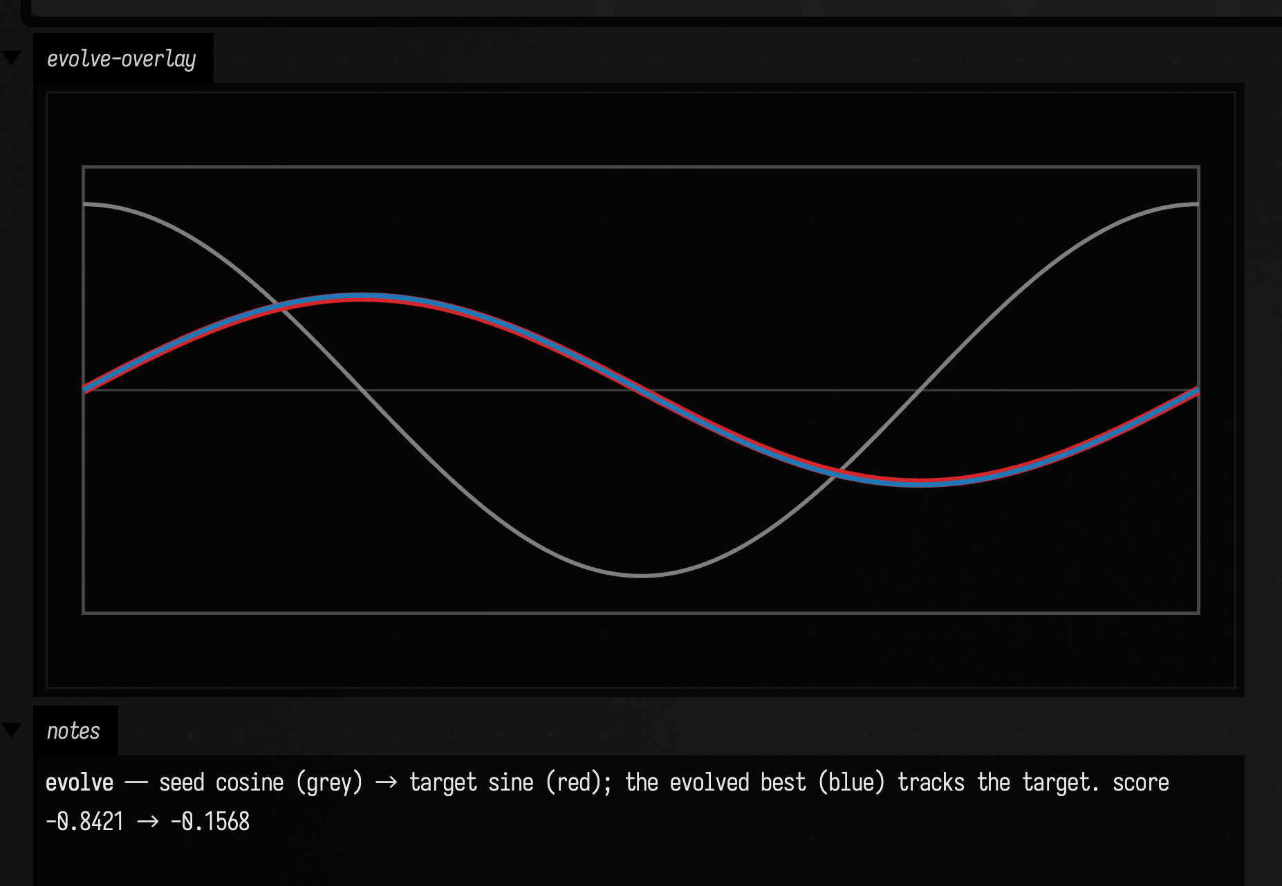
The grey curve is the seed cosine; the red curve is the target; the blue curve is run.best. The blue tracks the red almost exactly: the fitness (negative RMSE minus a small complexity penalty) climbs from −0.8421 at the seed to −0.1568 at the best, an ~81% reduction in error.
The order the accepted mutations arrive in is what each operator is for. The first one accepted is the structural leap: substituteOp turns the cosine into a sine and more than halves the error in a single step. From then on jitter and nudge walk the amplitude leaf down from 1.0 toward 0.5, interleaved with prune steps that shed now-redundant structure without hurting the fit, because the small complexityWeight rewards the simpler graph. The search stops improving well inside its 120-iteration bound, and every draw goes through one seeded Random, so it reproduces exactly. The iteration-by-iteration trace is in FUNCTIONS_EVOLVE_MEASUREMENTS.md.
Variety generation: novelty search for a set of gestures
matchFitness pulls every candidate toward one target. Often you want the opposite: a diverse family of gestures rather than one best match. evolveVariety(...) grows a behaviourally distinct set by novelty search, reusing the same evolve machinery and the same seeded-Random determinism.
Novelty is measured on a behavioural coordinate: what a graph does, not how it is built. Fn.behaviour(domain, samples) samples evalSafe on an even grid into an FnBehaviour descriptor (with a distanceTo), the counterpart to the structural view from graphMetrics. noveltyFitness(archive, ...) then rewards a candidate for being far (mean of its k-nearest neighbours) from an archive of already-seen behaviours. It is a drop-in (Fn) -> Double you can hand to plain evolve. evolveVariety orchestrates it: each slot evolves against a growing archive, adopts the winner, and drifts the seed onto it so the next slot has rich material to mutate away from.
val variety = evolveVariety(
    seed = sin(2.0) * 0.5,
    count = 6, // how many mutually-distant gestures to return
    iterations = 48,
    rngSeed = 7L, // same seed + inputs -> identical set
    neighbours = 3, // k-nearest novelty
    normalize = true, // measure distance in *shape*, not amplitude (see below)
)
println("spread = ${variety.meanPairwiseDistance}")
variety.results.forEachIndexed { i, fn -> fn.browseGraph(channel = "variety-$i") }
FnVarietyRun exposes the results, their behaviours, the per-slot runs, and
meanPairwiseDistance, the average distance across the set. Novelty is scored from sampled
behaviour, so the returned functions differ in what they do. Run it again with the same rngSeed
and inputs to reproduce the family.
Shape vs amplitude: the normalize flag
The metric that measures the distance decides whether variety search gives you a family or a single runaway. By default behaviour(...) records the raw sampled signal, so distanceTo measures distance in value space. Under that metric the cheapest way for a candidate to look "novel" is simply to be louder: scale an amplitude and you are far from everything in the archive without changing the gesture at all. Left unchecked, a novelty run drifts toward ever-bigger magnitudes, one gesture that blows up and the rest collapsed against it.
Passing normalize = true z-scores each descriptor (subtract the mean, divide by the RMS) before measuring distance, so amplitude and offset fall out and novelty has to explore shape instead: sine versus saw versus pulse versus something pruned flat. That also tames the default mutation palette, because duplicateSubtree only rescales a copy and normalization ignores a rescaling. Read it as the counterpart of the structural cost from graphMetrics: one asks "how big is the graph", the other "how different is what it does".
evolveVariety with normalize = true, run live in a box. Each slot's stored z-scored behaviour is drawn as an FLine in its own cell of a 3×2 montage, so all six cells share one scale and read as pure shape:
:::static
with(Functions) {
    /*
    Same run as the harness: grow 6 behaviourally distinct gestures from one seed by
    novelty search. normalize = true measures distance in *shape*, not amplitude, so
    the set spreads across genuinely different waveforms. Fixed rngSeed = 7L.
    */
    val variety = evolveVariety(
        seed = sin(2.0) * 0.5,
        count = 6,
        iterations = 48,
        rngSeed = 7L,
        samples = 120,
        neighbours = 3,
        normalize = true,
    )

    val cols = 3
    val cellW = 300.0
    val cellH = 180.0
    val gap = 20.0
    val topPad = 44.0
    val out = mutableListOf<FLine>()

    /*
    One mini-plot per result, laid out in a grid. Plot the stored *normalized*
    behaviour (variety.behaviours[i].samples) so every cell shares one z-scored
    scale and the montage reads as pure shape variety, not "the same wave rescaled".
    */
    variety.behaviours.forEachIndexed { i, b ->
        val col = i % cols
        val row = i / cols
        val cx0 = gap + col * (cellW + gap)
        val cy0 = topPad + row * (cellH + gap)
        val cyc = cy0 + cellH / 2
        val amp = (cellH / 2 - 12) / 2.6 // z-scored signal spans roughly +/-2.6

        out += fline {
            moveTo(cx0, cy0)
            lineTo(cx0 + cellW, cy0)
            lineTo(cx0 + cellW, cy0 + cellH)
            lineTo(cx0, cy0 + cellH)
            lineTo(cx0, cy0)
            color = vec(1.0, 1.0, 1.0, 0.22)
            thickness = 1.2
        }
        out += fline {
            moveTo(cx0, cyc)
            lineTo(cx0 + cellW, cyc)
            color = vec(1.0, 1.0, 1.0, 0.18)
            thickness = 1.0
        }
        val s = b.samples
        val curve = FLine()
        for (k in s.indices) {
            val px = cx0 + 8 + (cellW - 16) * k / (s.size - 1).toDouble()
            val py = cyc - amp * s[k]
            if (k == 0) curve.moveTo(px, py) else curve.lineTo(px, py)
        }
        curve.color = vec(0.12, 0.47, 0.71, 1.0)
        curve.thickness = 2.2
        out += curve
    }

    lines(out, channel = "evolve-variety", w = 980.0, h = 440.0, fitToSize = false)
    markdown(
        "notes",
        "**evolveVariety** — ${variety.results.size} behaviourally distinct gestures from one seed, meanPairwiseDistance ${variety.meanPairwiseDistance.f3} (normalized shape)",
    )
    variety
}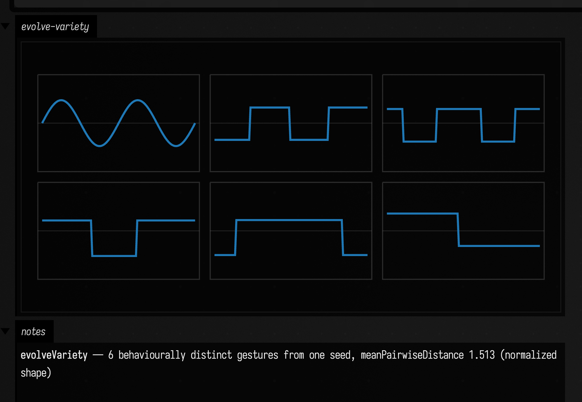
Six slots grown from a single sin(2.0) * 0.5 seed, meanPairwiseDistance = 1.51 across the set: every cell is a different shape, not the same wave rescaled. Run the same thing without normalize and the reported spread is far larger while the montage degenerates to one spike, because in value space the cheapest way to be novel is to be loud.
Replay it live. A loadable operation transcript, assets/evolve/variety-evolution.operations.yaml, builds and runs this in a fresh Field document: one box that grows the set and plots each gesture. Replay it with field_backdoor.py --scratch (macro write … && macro run …) or hand the YAML to the field_run_transcript MCP tool. See Automating Field for the transcript path.
Rewrite plot example
This example rewrites a nested graph in two ways: it changes a descendant saw into a triangle, then uses Kotlin RHS code to scale numeric values under sin by depth.
:::static
// A rewrite with @{...} blocks compiles them in this box, so it runs after the box's code has
// finished: go { } starts once this run returns.
go {
    with(Functions) {
        val base = (sin(sin(saw(0.18))) * 0.45) over (0.0..0.4)
        val changed =
            base.rewriteKotlin(
                """
#fnrewrite
sin/*/saw => op=triangle
sin/**/[tag=number][value>0.15] => *= @{1.0 + depth * 0.08}
**/[role=amplitude] => *= @{if (parentOp == "sin") 0.75 else 1.0}
""",
            )
        base.withName("before rewrite").plot(0.0..0.4, channel = "before", heightPx = 240, title = "before rewrite")
        changed.withName("after rewrite").plot(0.0..0.4, channel = "after", heightPx = 240, title = "after rewrite")
        (changed - base)
            .withName("rewrite delta")
            .plot(0.0..0.4, channel = "delta", heightPx = 220, title = "after - before")
    }
}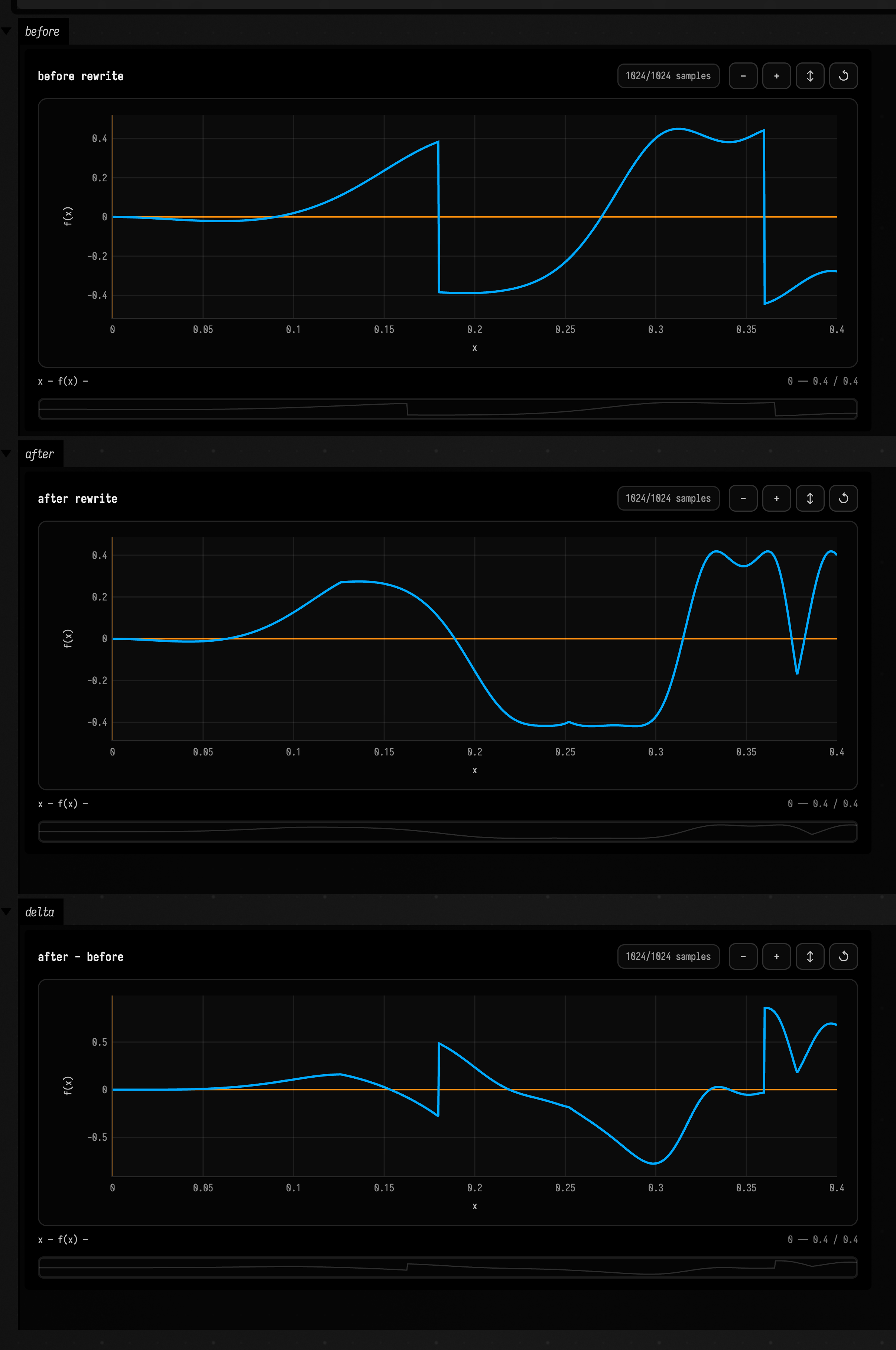
The selectors talk about structure, not sample values. The rules do not ask "where is the waveform high?"; they ask "which function graph nodes sit under this ancestry, role, or metadata condition?" Plotting the source, result, and delta over the first 0.4 units, before the nested sin starts oscillating faster than the plot can draw, puts the structural edit on screen: the graph rewrite is not only metadata, it changes the sampled signal.
Rewrite limitations
The graph is a recipe, not a decompiler. Standard Functions constructors and combiners participate because they attach graph metadata and rebuild functions. Raw fn { ... } lambdas are opaque: they can be copied as evaluators and shown as opaque nodes, but they cannot be structurally edited from the inside.
Path matching follows occurrence paths through the copied graph. This is what makes selectors like sin/**/[role=frequency] useful, but it also means shared subgraphs need a conscious choice. Leave preserveSharing = false for independent occurrence edits; pass preserveSharing = true when identity sharing matters more than path-specific mutation.
Finally, rewrite rules run during graph copy, bottom-up through children before parents. A rule can affect what later actions on the same node see, but it does not retroactively revisit children that have already been copied.
Notes
- 1D use-case: build one Fn stack and call toFLine.
- 2D use-case: build x(t) and y(t) stacks, then sample into a path FLine.
- Start with the simplest constructor that expresses the shape you want, then add modulation, windowing, and clipping only as needed.
- When a stack starts to feel hard to read, draw intermediate stages side by side instead of hiding everything inside the final curve.
Where the pictures come from
Every figure on this page is executed by the docs build: each is a diffstatic_runner fence, so the
image or video under it is that box's own output, drawn with lines(...) like everything else here.
The convergence video is a launched box whose loop runs one truncated fitGradient per frame.
The public declarations used on this page are listed, with their KDoc, in the codebase reference: Functions.kt. Start from what's already in the box.