Charts as FLines

A Chart is a plot made of FLines. Put one in the same drawing as your other FLines, click its marks, or draw an expected range and see which data falls outside it. For a general-purpose interactive chart, take a look at Plotly too.

New to Field's ways of displaying data? Looking at Data starts with values and plots in a box. If your data is already a table, DataFrames in a Box shows how to work with its columns.

You build a Chart up a call at a time and hand it to showChart. showChart(c), display(channel, c), c.h, and a box whose last expression is a Chart all render the same figure. Here is a residual curve with an expected bound:

Chart(title = "residual per iteration", xLabel = "iteration", yLabel = "|r|")
    .line("residual", iterations, residual)
    .points("residual", iterations, residual)
    .expect(max = 1e-6, because = "converged below 1e-6")

Reach for Plotly first

Field already has Plotly: linePlot, scatter, violin, showSignals, each described in the reference under plotly.kt. The shortest of them puts named signals on screen in one call:

showSignals("residual" to residual, "step" to step, title = "per iteration")

The others return a Plot for you to display; DoughDSP: hear the primitives uses showSignals throughout. Plotly has real text, a legend with line swatches, axes that autorange, and it reflows to whatever shape you give it. A Chart is fixed geometry fitted and centred in its panel, so a panel of a different shape leaves empty margin, and its text scales with the figure.

Use a Chart instead when you need one of these:

• the plot drawn under the same transform as other FLine geometry, which Plotly cannot join;
• clicking a mark and getting back the datum it stands for;
• expect(), which draws an expected range on the plot.

The marks

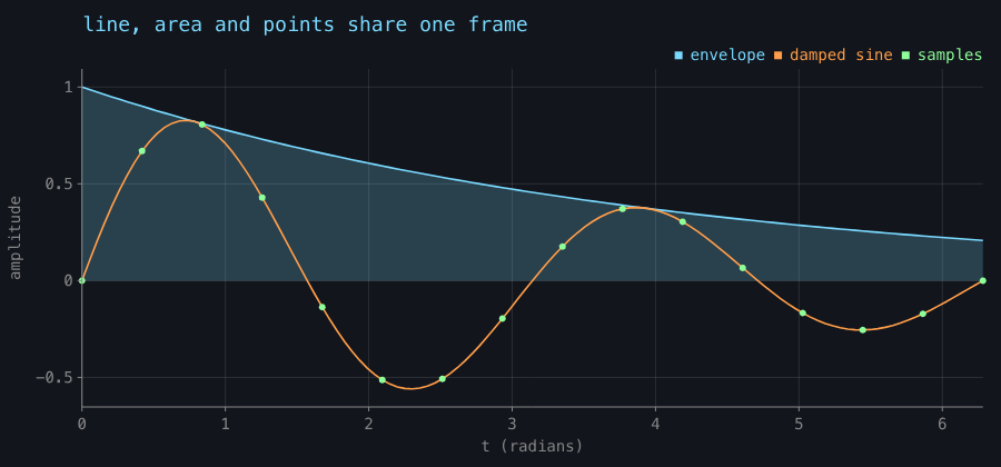
points, line, area, bars, histogram, plus rule, vrule and band for annotation. Marks over the same numbers share one frame and one legend.

val xs = (0..120).map { it / 120.0 * 6.28318 }
val decay = xs.map { exp(-it * 0.25) * sin(it * 2.0) }
val envelope = xs.map { exp(-it * 0.25) }

Chart(title = "line, area and points share one frame", xLabel = "t (radians)", yLabel = "amplitude")
    .area("envelope", xs, envelope)
    .line("damped sine", xs, decay)
    .points(
        "samples",
        xs.filterIndexed { i, _ -> i % 8 == 0 },
        decay.filterIndexed { i, _ -> i % 8 == 0 },
    )

bars takes categories and puts them on the axis, so you do not index them yourself:

Chart(title = "bars put their categories on the axis", yLabel = "gates")
    .bars("cost", ["xor", "maj3", "adder", "mux", "parity"], [6, 11, 27, 4, 19])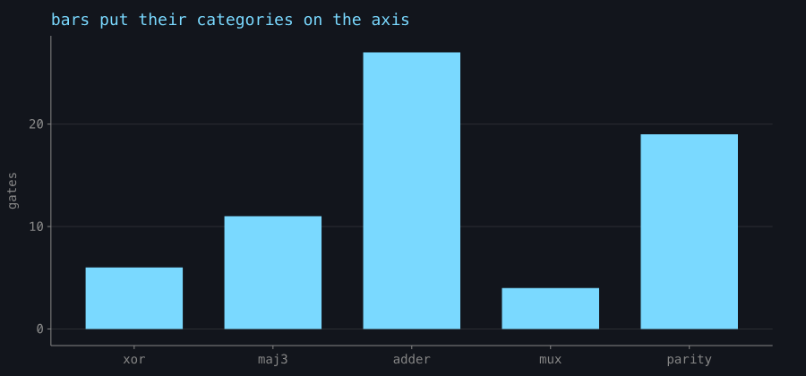

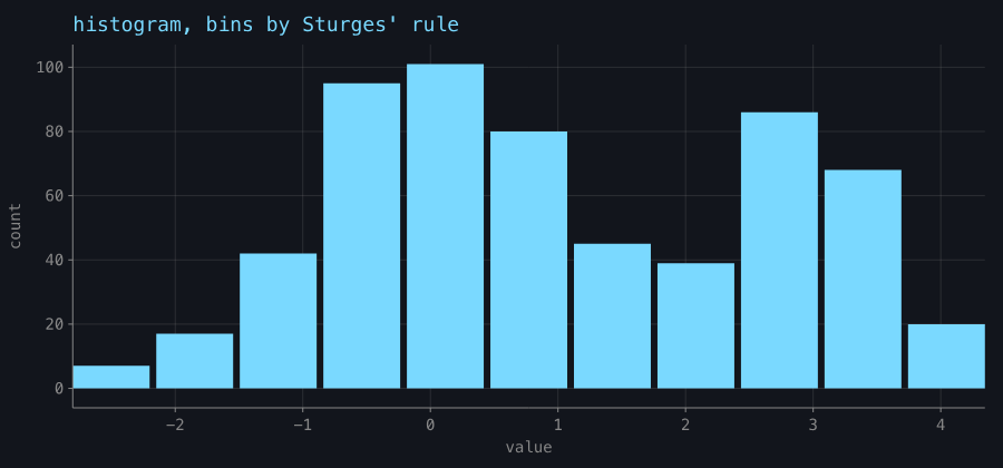
histogram bins for you by Sturges' rule:

Scales and ticks

Scale(lo, hi, pixelLo, pixelHi, kind) maps data to pixels with toPixel/toData. A y scale is built inverted, because y grows downwards in Field's 2D outputs.

The tick functions are public, so you can use them for an axis of your own: niceTicks(lo, hi, target), logTicks, niceNumber, tickLabel and tickLabels.

Values are snapped to their own step, so an axis never reads 0.30000000000000004, and tickLabels picks one notation for a whole axis rather than per label.

Set xKind/yKind to ScaleKind.LOG for a log axis. A log scale refuses a non-positive domain, and a non-positive datum is left out of the plot.

val n = (1..6).map { 10.0.pow(it) }
val time = n.map { it * 1.4e-6 + 3e-4 }

Chart(title = "a log axis, and decade ticks", xLabel = "n", yLabel = "seconds")
    .also {
        it.xKind = ScaleKind.LOG
        it.yKind = ScaleKind.LOG
    }
    .line("measured", n, time)
    .points("measured", n, time)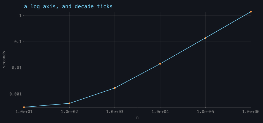

expect(): drawing what the data should do

expect(min, max, series, because) draws the expectation: the accepted range becomes a band across the plot, the bounds it names are ruled, data outside recolours, and the footnote counts the violations. An unbounded side draws no edge, which is the visual difference between "at most 1e-6" and "between 0 and 1e-6".

Chart(title = "residual per iteration", xLabel = "iteration", yLabel = "|r|", note = "Adam, lr 0.05")
    .line("residual", iterations, residual)
    .points("residual", iterations, residual)
    .expect(max = 1e-6, because = "converged below 1e-6")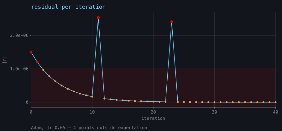

• Chart.deviations returns the points outside the expectation, so a test can assert on the same list the footnote counts. There is also a predicate form, expect(series, because) { x, y -> … }, with no shape to draw.
• Each datum is counted once. A line for the trend plus points to make it clickable is two marks over one datum, and the footnote counts that datum once.

Picking marks

Box.lines switches to the interactive SVG renderer the moment any line carries onClick or hoverColor. Point and bar marks set both, plus a label naming the datum, so you can hover over a bar or click a point with no extra setup:

val c = Chart(yLabel = "gates").bars("cost", "xor" to 6, "adder" to 27)
c.onPick = { pick ->
    print("${pick.series}/${pick.category} = ${pick.y}")
}
showChart(c)

Set pickable = false to turn this off. A series with more data than pickLimit (400 by default) stops responding point by point.

From a DataFrame

DataFrame<*>.chart() picks the axes so you do not have to name them for a quick look: the first numeric column for x if the frame has two or more, otherwise the first column as categories, otherwise the row index; then every remaining numeric column as a series.

import org.jetbrains.kotlinx.dataframe.api.*

val people = dataFrameOf("name", "age")("Alice", 15, "Bob", 30, "Cara", 45)

people.chart() // bars: age per name
people.chart(x = "name", y = ["age"]) // choose both axes explicitly
showChart(people) // straight from a frame to the screen

import org.jetbrains.kotlinx.dataframe.api.*

val people = dataFrameOf("name", "age")("Alice", 15, "Bob", 30, "Cara", 45)

showChart(people) // bars: age per name, chosen by chart()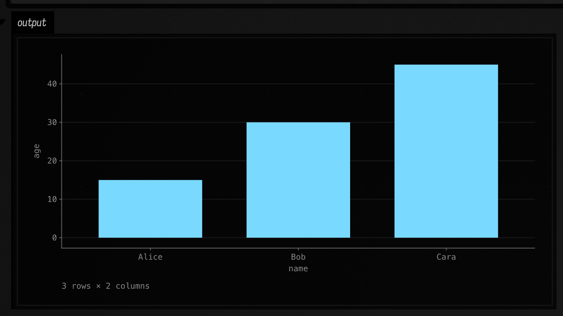

Series are capped for auto-selection, because a legend stops being readable past a handful of entries, and the per-datum dots are dropped automatically for a frame with more rows than pickLimit. See DataFrames in a Box.

Keeping a figure inside its frame

The panel a Chart lands in is fitted to the geometry it actually draws, so anything drawn outside width × height would make the whole figure smaller. clip, on by default, prevents that in two ways:

• mark geometry is cut to plotRect: lines and area outlines by Liang–Barsky, an area's fill by Sutherland–Hodgman so it stays closed, a point outside dropped whole, a bar clamped on both axes and dropped when no part of it is in the window, a rule or a band that falls off the axis not drawn at all. A clipped series stays one FLine with several subpaths, so it is still one series, one legend entry, and one thing to hover;
• title and note are wrapped to the figure width, capped at two and four lines with an ellipsis past that.

Clipping only matters when you set an explicit xDomain or yDomain, because a derived domain always covers its own data.

The same marks in an explicit window, with clip off and then on:

// The same marks in an explicit window, with clip off and then on.
fun figure(clipped: Boolean) =
    Chart(title = if (clipped) "clip = true" else "clip = false", xLabel = "x", yLabel = "y")
        .area("area", (0..40).toList(), (0..40).map { it * 0.6 - 6.0 })
        .line("line", (0..40).toList(), (0..40).map { 22.0 - it * 0.9 })
        .points("points", (0..40).toList(), (0..40).map { 4.0 + it * 0.4 })
        .apply {
            xDomain = 8.0 to 32.0
            yDomain = 0.0 to 20.0
            clip = clipped
        }

showChart(figure(false), channel = "unclipped")
showChart(figure(true), channel = "clipped")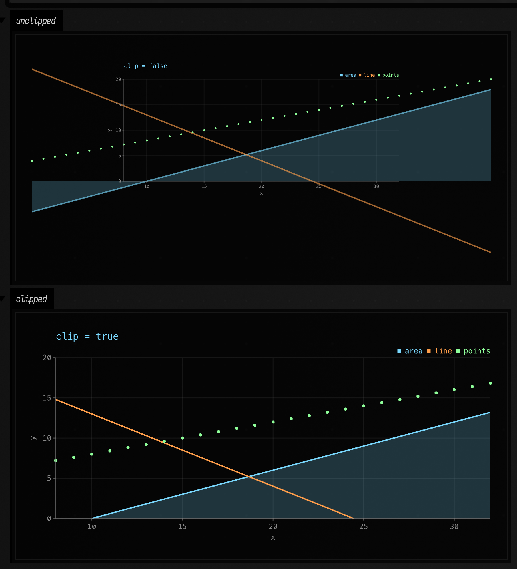

Set clip = false when you are composing a chart with other FLine geometry under a shared transform and want the overflow.

Down to geometry

toFLines() lowers the whole figure to List<FLine> in pixel space and plotRect() reports the rectangle the marks are clipped to, so the chart can go into the same drawing as the rest of your geometry, under one transform. toHTML() goes through afield.ui.visualization.linesToHTML, the same markup Box.lines builds.

Labels are glyph outlines. On a machine with no fonts, the chart is drawn without labels.

Text of your own goes in as TextLayout.toFLines() (one line per glyph) or toFLine() (one for the whole string). Move it with FLine.transform, which carries each curve's control points with its end points.

CHART_GALLERY_DIR=public/docs/assets/chart_gallery python3 tools/run_field_tests.py --id visualization.chart-gallery

./gradlew jvmTest --no-daemon --tests 'afield.ui.visualization.ChartTest'

Reference

The generated API listing is under Visualization. See also DataFrames in a Box and FLine examples.