Measuring dependence between two signals
You have two streams of numbers and want to know whether they are related. Field's tools for that
live in the afield.math.statistics package, in three files:
stats.kt,
correlations.kt
and
quantilewarp.kt.
This page works through all three. Each dependence coefficient answers a slightly different version of the question, so the page shows which one to use for which
kind of relationship.
stats.kt has the summary statistics: count, quartiles, IQR, MAD, skew, kurtosis, histograms and
a streaming window of all of it. correlations.kt has the dependence coefficients: Pearson,
Spearman, Kendall, Chatterjee's xi, distance correlation, a MIC-like grid scan, and rolling
versions of the last two. quantilewarp.kt reshapes a signal's distribution into one you
choose, for when a signal has the wrong shape to work with.
Where the family lives
| what you want | where it is | notes |
|---|---|---|
| count, quartiles, IQR, MAD, variance, skew, excess kurtosis | stats.kt |
buildSummaryStats → SummaryStats. Non-finite input is dropped and counted |
| a streaming window of all of that | stats.kt |
SummaryStatsBuffer, plus Vec2/Vec3/Vec4SummaryStatsBuffer which add per-component stats, vector length and the pairwise component correlations |
| histograms | stats.kt |
buildHistogram → Histogram / HistogramBin |
| those, rendered | stats.kt |
histogramToSvg, seriesPlotToSvg, summaryStatsBoxToHtml — string-interpolated SVG/HTML, no drawing library, cyan-on-black by default |
| the dependence coefficients | correlations.kt |
StatsDependence.pearson / spearman / kendallTauB / chatterjeeXi (aliased xi) / distanceCorrelation / micTicNaive |
| dependence over a sliding window | correlations.kt |
RollingDistanceCorrelation (incremental, O(w) per sample), RollingXiCorrelation (recomputes, O(w log w) per sample) |
| reshape a distribution into a target | quantilewarp.kt |
AdaptiveQuantileWarp, QuantileWarpState, TargetDistributions, inverseStandardNormalCdf, and matching GLSL for the GPU |
There are no p-values, confidence intervals or hypothesis tests in these files. Whether a number
means anything is yours to establish, and Measuring the null yourself below writes the
permutation test that does it. Note too that micTicNaive is not MICe/TICe. The file's own header comment
(correlations.kt:36) says it is an equipartition-grid approximation that will not
reproduce published numbers.
Values Over Time has a shorter version of the dependence examples, next to the interpolants.
Summary statistics
buildSummaryStats takes any Iterable<Double> and hands back seventeen numbers.
SummaryStatsBuffer wraps it in a synchronized, capped sliding window you can add to sample by
sample, and summaryHtml() renders the whole thing (metrics, histogram and series plot) as one
self-contained HTML card.
:::static
// A right-skewed signal by construction: exp of a Gaussian, so we know the shape we are asking about.
val rng = java.util.Random(11)
val signal = (0 until 500).map { exp(0.6 * rng.nextGaussian()) }

val buf = SummaryStatsBuffer(maxSize = 500)
buf.addAll(signal)
buf.add(Double.NaN) // dropped, and counted, at `add` time
buf.add(Double.POSITIVE_INFINITY) // likewise: `values` never holds a non-finite number

val s = buf.snapshot()

/*
Three things the card reports that are easy to misread, pinned here as arithmetic:
 - MAD is the *median absolute deviation from the median*, unscaled. For a normal sample it is
   about 0.6745 sigma, not sigma; here the signal is skewed, so it is smaller than the IQR/2.
 - `range` is max - min, which for a skewed signal is dominated by the single largest sample.
 - `cv` is sampleStdDev / mean, so it is meaningless the moment the mean crosses zero.
*/
val madOverIqr = s.mad / s.iqr
val note =
    "n=${s.count}, dropped=${s.droppedCount}; " +
        "median=${s.median.f3}  mean=${s.mean.f3} (mean > median: right-skewed); " +
        "MAD=${s.mad.f3} = ${madOverIqr.f3} x IQR; " +
        "skew=${s.skewness.f3}  excess kurtosis=${s.kurtosisExcess.f3}"
:::fold render the card
display("card", buf.summaryHtml(widthPx = 620, chartHeightPx = 150, decimals = 3))
markdown("read this off the card", "{muted:$note}", width = 620)
:::endfold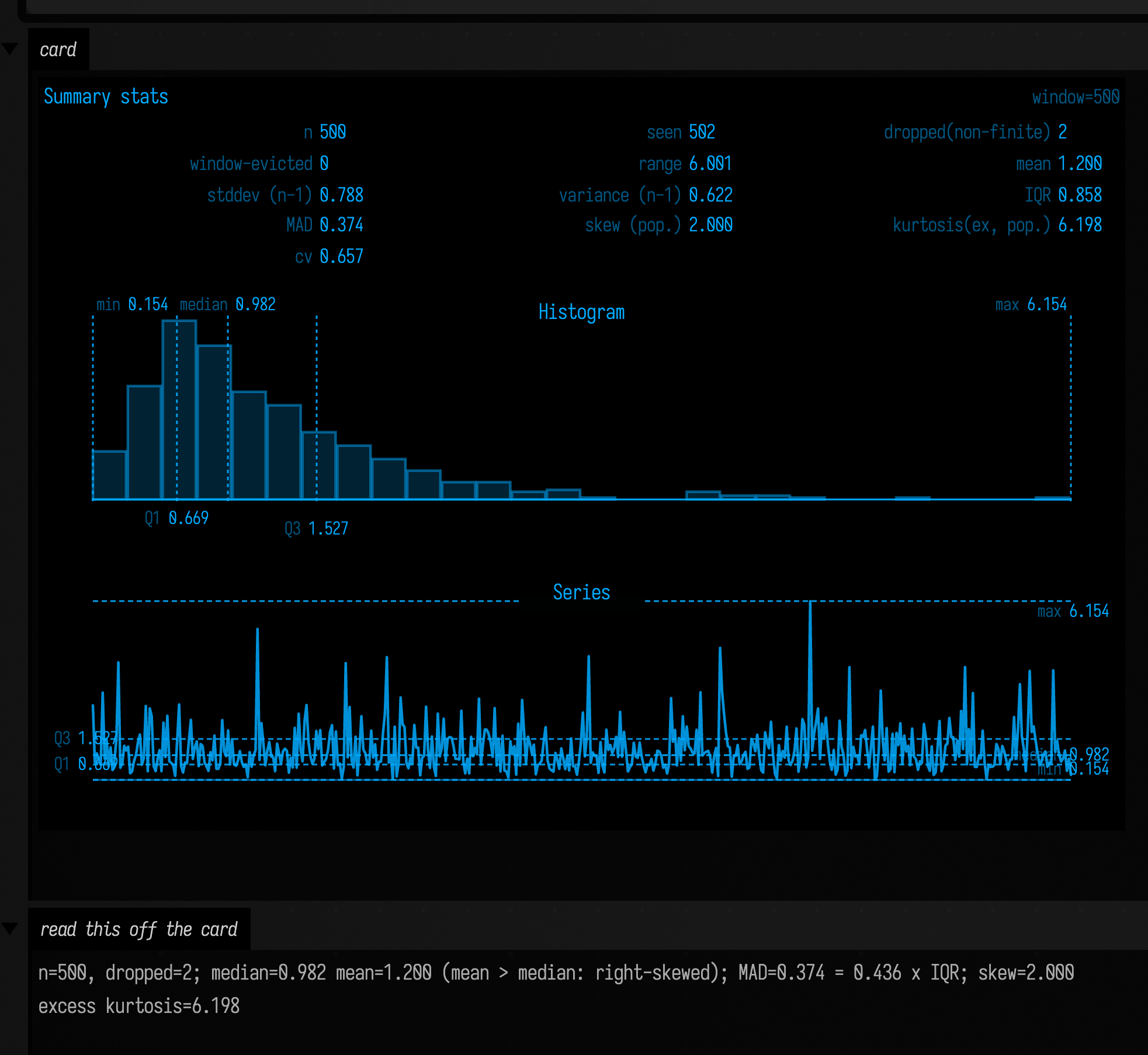
Each label on the card names its convention: stddev (n−1) and variance (n−1) are the
sample forms, skew (pop.) and kurtosis(ex, pop.) the population forms, with no bias
correction. If you are comparing against another tool, the mapping onto NumPy and SciPy is exact: q1/median/q3 are
numpy.percentile's default linear interpolation, mad is \( \operatorname{median}(\lvert y - \operatorname{median}(y) \rvert) \) unscaled,
sampleStdDev is numpy.std(ddof=1), and skewness/kurtosisExcess are scipy.stats.skew and
scipy.stats.kurtosis at their default bias=True.
Agents: what pins the SciPy mapping
StatsSummaryTest pins that mapping to ten decimal places against SciPy 1.15.2 on a
tie-heavy ten-point sample.
Three more edges, guarded rather than propagated inside buildSummaryStats
(stats.kt:1004), so you get a
number instead of a NaN:
- one sample:
sampleVarianceis 0.0, not NaN; - two samples:
skewnessis 0.0; it needsn > 2; - three samples:
kurtosisExcessis 0.0; it needsn > 3.
SummaryStatsBuffer keeps two separate drop counters
(stats.kt:405).
dropped(non-finite) counts values it refused; window-evicted counts values that aged out of the
window. Feed 200 finite samples to a maxSize = 64 buffer and you get size=64, samplesSeen=200,
droppedByCapacity=136.
Histograms, and the rule that picks the bins
buildHistogram chooses its own bin width: the smallest of the Freedman–Diaconis, Scott and
Sturges estimates, floored at range/2000 so the bin count can never exceed 2000. "Smallest" means
finest, which is usually what you want. The fence below re-derives the whole decision from the
published SummaryStats and predicts the bin count before asking.
:::static
val rng = java.util.Random(11)
val skewed = (0 until 500).map { exp(0.6 * rng.nextGaussian()) }

// Two clean modes, 4 apart, each with sd 0.4 — the case the rule handles worst.
val rng2 = java.util.Random(23)
val bimodal =
    (0 until 500).map { if (it % 2 == 0) -2.0 + 0.4 * rng2.nextGaussian() else 2.0 + 0.4 * rng2.nextGaussian() }

/*
Re-derive the three candidate widths from the public stats and predict the bin count.
This shares `quantileSorted` with the implementation, so it checks the *rule selection and the
rounding* — not the quantiles themselves. Those are checked against SciPy in jvmTest instead.
*/
fun explain(name: String, values: List<Double>): String {
    val s = buildSummaryStats(values)
    val n = s.count
    val range = s.max - s.min
    val cubeRootN = n.toDouble().pow(-1.0 / 3.0)
    val hFd = 2.0 * s.iqr * cubeRootN // Freedman-Diaconis
    val hScott = 3.5 * s.sampleStdDev * cubeRootN // Scott
    val kSturges = ceil(ln(n.toDouble()) / ln(2.0) + 1.0).toInt() // Sturges
    val hSturges = range / kSturges
    val winner = minOf(hFd, hScott, hSturges)
    val which = when (winner) {
        hFd -> "Freedman-Diaconis"
        hScott -> "Scott"
        else -> "Sturges"
    }
    val predicted = Math.round(range / winner).toInt().coerceIn(1, 2000)
    val actual = buildHistogram(values)
    return "$name: FD=${hFd.f4}  Scott=${hScott.f4}  " +
        "Sturges=${hSturges.f4} (k=$kSturges) -> $which wins; " +
        "predicted ${predicted} bins of ${(range / predicted).f5}, " +
        "got ${actual.bins.size} of ${actual.binWidth.f5}; counts sum to ${actual.count}"
}

val skewedNote = explain("skewed", skewed)
val bimodalNote = explain("bimodal", bimodal)
:::fold draw both histograms
val svgs = [
    histogramToSvg(
        buildHistogram(skewed),
        widthPx = 470,
        heightPx = 270,
        padTop = 26,
        title = "exp(0.6 g), n=500",
        decimals = 3,
    ),
    histogramToSvg(
        buildHistogram(bimodal),
        widthPx = 470,
        heightPx = 270,
        padTop = 26,
        title = "two modes at -2 and +2, n=500",
        decimals = 3,
    ),
]
showRow("histograms", svgs)
markdown(
    "the rule, re-derived",
    """
    {muted:$skewedNote}

    {muted:$bimodalNote}
""",
    width = 960,
)
:::endfold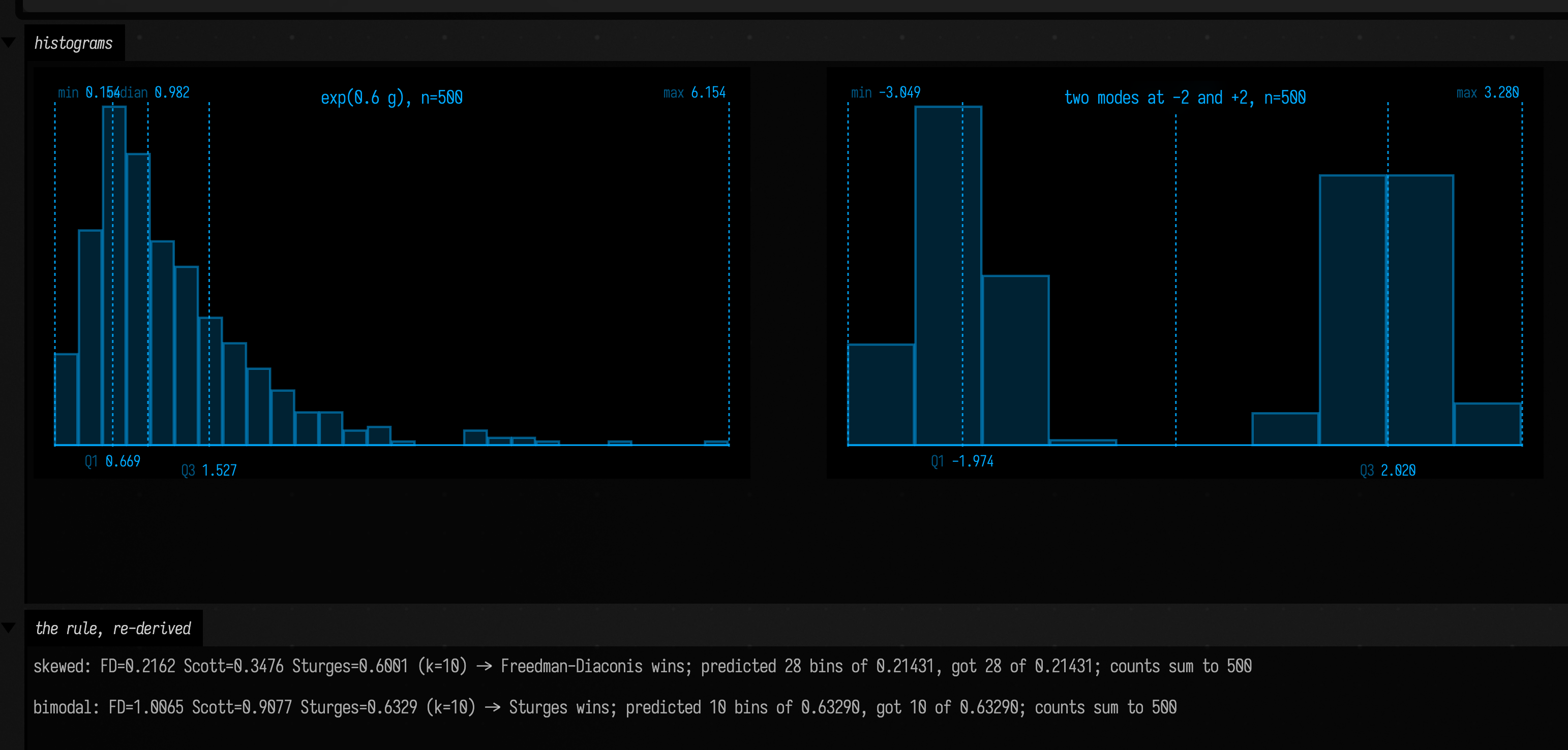
Both predictions land: 28 bins of 0.21431 for the skewed signal, 10 bins of 0.63290 for the bimodal
one, and in both cases the bin counts sum back to 500. Which rule won is the part to read. On the
skewed signal Freedman–Diaconis is the finest at 0.2162 and it decides. On the bimodal signal FD
comes out at 1.0065 and Scott at 0.9077 (both much coarser) because both are driven by
global spread, and here the spread is the distance between the modes (IQR 3.99, sample sd 2.06)
rather than the spread within them (0.4). Which leaves Sturges winning at 0.6329, and Sturges is
the one rule of the three that looks at nothing but n: \( \lceil \log_2 n + 1 \rceil \) is 10 bins for any
500-point sample whatever its shape. So a multi-modal signal falls back to the crudest of the three
estimates and its two obvious modes get about one bin each. buildHistogram takes no bin-count
argument (stats.kt:1214), so if you need finer bins for a signal
like this, bin it yourself.
Comparing the dependence coefficients
Every coefficient in StatsDependence takes two equal-length DoubleArrays and returns one
number, but they measure different things. This example draws six shapes of relationship and
prints every coefficient under each:
:::static
val n = 400
val rng = java.util.Random(7)
val x = DoubleArray(n) { it / (n - 1.0) * 2.0 - 1.0 } // an even sweep of -1..1
val noise = DoubleArray(n) { rng.nextGaussian() } // ONE noise draw, reused, so the
// "independent" panel is literally
// the noise the others are built on
val cases = [
    "linear" to DoubleArray(n) { 0.8 * x[it] + 0.25 * noise[it] },
    "monotone, curved" to DoubleArray(n) { exp(3.0 * x[it]) },
    "parabola" to DoubleArray(n) { x[it] * x[it] },
    "sine, 3 cycles" to DoubleArray(n) { sin(3.0 * PI * x[it]) },
    "same mean, growing spread" to DoubleArray(n) { (0.05 + abs(x[it])) * noise[it] },
    "independent" to DoubleArray(n) { noise[it] },
]

fun coefficients(y: DoubleArray): String {
    val d = "%.3f"
    return "r=${d.format(StatsDependence.pearson(x, y))}   " +
        "rho=${d.format(StatsDependence.spearman(x, y))}   " +
        "tau=${d.format(StatsDependence.kendallTauB(x, y))}   " +
        "xi=${d.format(StatsDependence.xi(x, y))}   " +
        "dCor=${d.format(StatsDependence.distanceCorrelation(x, y))}   " +
        "MIC~=${d.format(StatsDependence.micTicNaive(x, y).mic)}"
}

:::fold draw the six panels
/*
Each panel is min-max rescaled into the unit square so the six share one window; SVG y grows
downward, so flip it to read the shapes the way the formulas are written.

Two columns because three panels this wide do not fit the capture, and the panels are worth
more here than a third column would be. A caption longer than `cellWidth` now wraps inside the
card instead of widening it out of frame — that used to cost you a whole column.
*/
val window = Rect(0.0, 0.0, 1.0, 1.0)
val frame = window.toFLine(color = vec(0.35, 0.44, 0.56, 0.5), thickness = 1.0)

val panels = cases.map { (name, y) ->
    val lo = y.min()
    val hi = y.max()
    val span = (hi - lo).takeIf { it > 1e-12 } ?: 1.0
    val cloud = pointCloudFLine(
        (0 until n).map { i -> vec((x[i] + 1.0) / 2.0, 1.0 - (y[i] - lo) / span) },
        color = vec(0.48, 0.85, 1.0, 0.8),
        pointSize = 1.1,
    )
    "$name\n${coefficients(y)}" to [frame, cloud]
}

showPlaneGrid(
    *panels.toTypedArray(),
    columns = 2,
    cellWidth = 430,
    cellHeight = 262,
    window = window,
)
:::endfold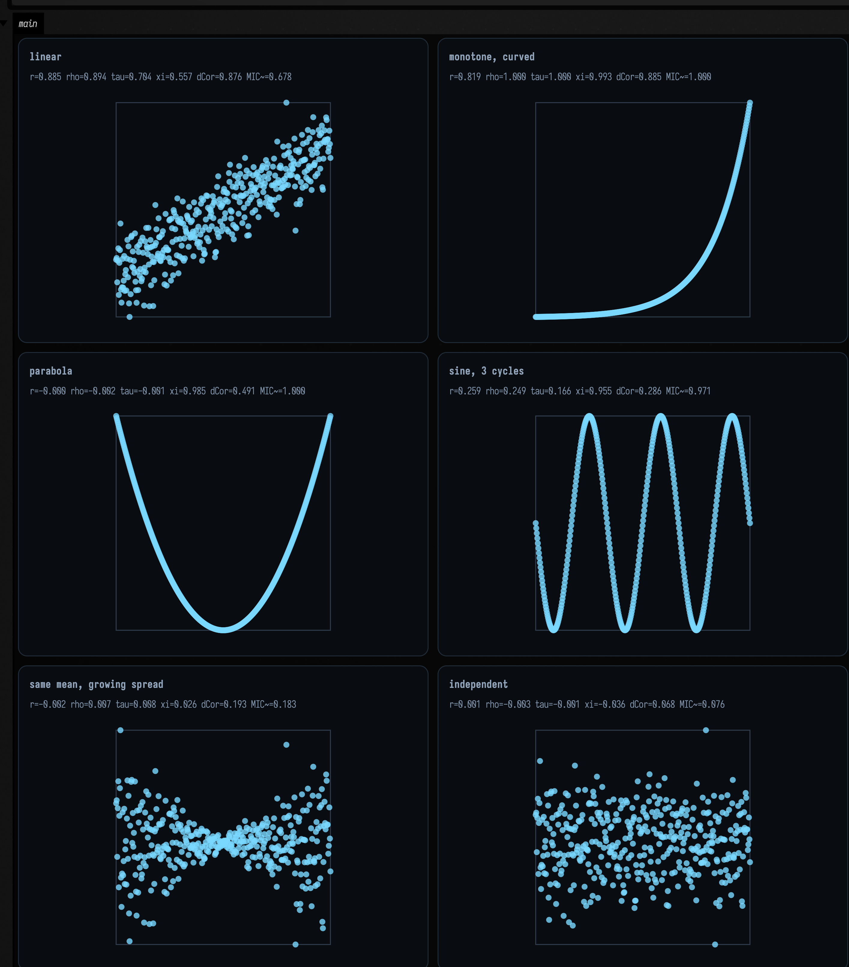
Read the captions across the grid, or the same numbers as a table:
| shape | pearson |
spearman |
kendallTauB |
xi |
distanceCorrelation |
micTicNaive().mic |
|---|---|---|---|---|---|---|
| linear | 0.885 | 0.894 | 0.704 | 0.557 | 0.876 | 0.678 |
monotone, curved (exp 3x) |
0.819 | 1.000 | 1.000 | 0.993 | 0.885 | 1.000 |
| parabola | −0.000 | −0.002 | −0.001 | 0.985 | 0.491 | 1.000 |
| sine, 3 cycles over x = −1..1 | 0.259 | 0.249 | 0.166 | 0.955 | 0.286 | 0.971 |
| same mean, growing spread | −0.002 | 0.007 | 0.008 | 0.026 | 0.193 | 0.183 |
| independent | 0.001 | −0.003 | −0.001 | −0.036 | 0.068 | 0.076 |
The table says which measure to use for which question.
Pearson answers "is this a straight line", and nothing else. r = −0.000 on the parabola,
where y is a noiseless, exact function of x: the dependence is total and the coefficient is
zero. pearson (correlations.kt:152) is the sample covariance over the
product of the standard deviations, and a symmetric parabola has zero covariance with its own
argument by construction.
Spearman and Kendall answer "is this monotone". They hit exactly ±1 on exp(3x) where Pearson
reads 0.819, which is the whole reason they exist: any strictly increasing reshape of y leaves
them alone. But they side with Pearson on the parabola, and for the same reason: a parabola is a
function and not a monotone one, and monotone is all either of them can see. spearman is literally
pearson on ranksAverageTies (correlations.kt:176–correlations.kt:181), so it inherits every
Pearson limitation after the ranking.
Chatterjee's xi answers "is y a function of x", and it is the only asymmetric coefficient
here. It reads 0.985 on the parabola and 0.955 on the sine, the two cases the rank coefficients
miss entirely. Swap the arguments and it changes its mind: xi(x, parabola) = 0.985 but
xi(parabola, x) = 0.246, because x genuinely is not a function of \( x^2 \) — each y has two
possible x. Cheap, too: O(n log n) against the O(n²) of kendallTauB and distanceCorrelation.
Distance correlation answers "is there any dependence at all". It is the only entry in the
table that is non-zero on every dependent row, including the last interesting one: the
growing-spread panel, where y has the same mean everywhere and only its scale depends on x.
Pearson, Spearman and Kendall read 0.00 there. Xi is also small in this example (0.026); the relationship changes the spread of y rather
than making it a deterministic function of x. Distance correlation reads 0.193, and the
next section puts that against the null it would have to beat.
And the trap in reading distance correlation: it is not a measure of how strong the
dependence is. dCor is 1 only for an exactly linear relationship (distanceCorrelation(x, 3x+1) is
exactly 1.0, and so is distanceCorrelation(x, −2x+5); it is unsigned). On the parabola,
where y is a perfect function of x, it reads 0.491; on the sine, 0.286. A lower dCor need not mean a relationship is unimportant; its value depends on the shape and
distribution of the data. Use it to decide whether to keep looking, then use other views and
measures to describe what you found.
How xi handles a tied predictor
Chatterjee's estimator is only defined up to a random breaking of the ties among the x
values, so on tied x it is a random variable rather than a number. Rather than pick a seed,
chatterjeeXi returns that random variable's exact expectation, computed in closed form
from the ranks inside each run of equal x (correlations.kt:325–correlations.kt:353). So it
is deterministic, reproducible, and invariant to the order you hand the pairs over in.
Two consequences. A constant predictor reads 0: for a single tie group the numerator's
expectation is \( (n^2-1)/3 \) against a denominator of \( n(n^2-1)/3 \), so the closed form is exactly
zero for every n. In Double it is zero to within one ulp rather than bit-exact, so compare
it against a tolerance, not against 0.0; dev_docs/STATISTICS_MEASUREMENTS.md has the sweep
that bound comes from. And a quantised predictor (a bucketed index, an integer
control value, a thresholded signal) is answered correctly: heavy ties with a real relationship
still read high (a ten-block staircase reads 0.891), while heavy ties with no relationship
read ~0.
Inputs whose x values are all distinct are unaffected, bit for bit, so every number elsewhere
on this page is a tie-free case. Every other coefficient here refuses a constant outright:
pearson, spearman and kendallTauB return NaN, and distanceCorrelation returns 0.0.
Agents: xi values recorded before 2026-07-30
Recorded xi values on tied x from before 2026-07-30 are wrong, not merely different:
x-ties then broke by input index, which scored how nearly y was a function of the order the
samples arrived in. dev_docs/stdlib_behaviour_changes.md owns that history and the
chatterjeeXi KDoc points at it.
Measuring the null yourself
There are no p-values in this family. That matters most for distance correlation, because dCor
under genuine independence is not 0 at finite n: the estimator is biased upward, and the bias
is large enough to swamp a real effect if you do not know its size. The independent row above
reads 0.068 at n=400; shrink the sample and the bias grows fast, and by n=25 the null's 95th
percentile is up at 0.466.
So measure the null yourself. Re-pair y against x at random a few hundred times, and see where
the number you actually observed falls:
:::static
val n = 400
val x = DoubleArray(n) { it / (n - 1.0) * 2.0 - 1.0 }
val rng = java.util.Random(7)
val noise = DoubleArray(n) { rng.nextGaussian() }
val y = DoubleArray(n) { (0.05 + abs(x[it])) * noise[it] } // the growing-spread panel again

val observedDcor = StatsDependence.distanceCorrelation(x, y)
val observedXi = StatsDependence.xi(x, y)

// The null: break the pairing, keep both marginals. Anything left is chance.
val prng = java.util.Random(31)
val reps = 400
val order = (0 until n).toMutableList()
val nullDcor = DoubleArray(reps)
val nullXi = DoubleArray(reps)
for (r in 0 until reps) {
    order.shuffle(prng)
    val shuffled = DoubleArray(n) { y[order[it]] }
    nullDcor[r] = StatsDependence.distanceCorrelation(x, shuffled)
    nullXi[r] = StatsDependence.xi(x, shuffled)
}
val sortedD = nullDcor.sortedArray()
val p95 = sortedD[(reps * 0.95).toInt()]
val exceed = sortedD.count { it >= observedDcor }
val xiExceed = nullXi.count { it >= observedXi }

// How large does dCor have to be before it means anything? Measure the null's 95th percentile
// against n, and against a fitted 2.5/sqrt(n).
val sizes = [25, 50, 100, 150, 200, 300, 400]
val thresholds = sizes.map { m ->
    val r2 = java.util.Random(1234)
    val k = 150
    val v =
        DoubleArray(k) {
                StatsDependence.distanceCorrelation(
                    DoubleArray(m) { r2.nextGaussian() },
                    DoubleArray(m) { r2.nextGaussian() },
                )
            }
            .sortedArray()
    v[(k * 0.95).toInt()]
}
val fitted = sizes.map { 2.5 / sqrt(it.toDouble()) }
// Plotted against 1/sqrt(n) rather than n: it turns the claim into a straight line through the
// origin, which is a much stronger thing to see than a hyperbola.
val inverseRootN = sizes.map { 1.0 / sqrt(it.toDouble()) }
:::fold two figures
val hist = buildHistogram(nullDcor.toList())
showSignals(
    "dCor over $reps random re-pairings" to hist.bins.map { it.count },
    x = hist.bins.map { (it.start + it.end) / 2.0 },
    channel = "null at n=400",
    title = "The null distribution of dCor, and where the observed value sits",
    xTitle = "distance correlation",
    yTitle = "count",
    marks = [
        "null 95th pct = ${p95.f3}" to p95,
        "observed = ${observedDcor.f3}" to observedDcor,
    ],
)
showSignals(
    "measured 95th pct of the dCor null" to thresholds,
    "2.5 / sqrt(n)" to fitted,
    x = inverseRootN,
    channel = "threshold vs n",
    title = "How big dCor has to be to mean anything: proportional to 1/sqrt(n)",
    xTitle = "1 / sqrt(n)   (n=400 left, n=25 right)",
    yTitle = "dCor",
)
markdown(
    "verdict",
    """
    {muted:observed dCor = ${observedDcor.f4}; null mean ${nullDcor.average().f4},
    95th pct ${p95.f4}, max ${sortedD.last().f4};
    re-pairings reaching the observed value: $exceed / $reps}

    {muted:observed xi = ${observedXi.f4}; xi null 95th pct
    ${nullXi.sortedArray()[(reps * 0.95).toInt()].f4};
    re-pairings reaching it: $xiExceed / $reps}

    {muted:null 95th pct vs n (measured / 2.5-over-root-n):
    ${sizes.indices.joinToString(" · ") { "n=${sizes[it]} ${thresholds[it].f3}/${fitted[it].f3}" }}}
""",
    width = 900,
)
:::endfold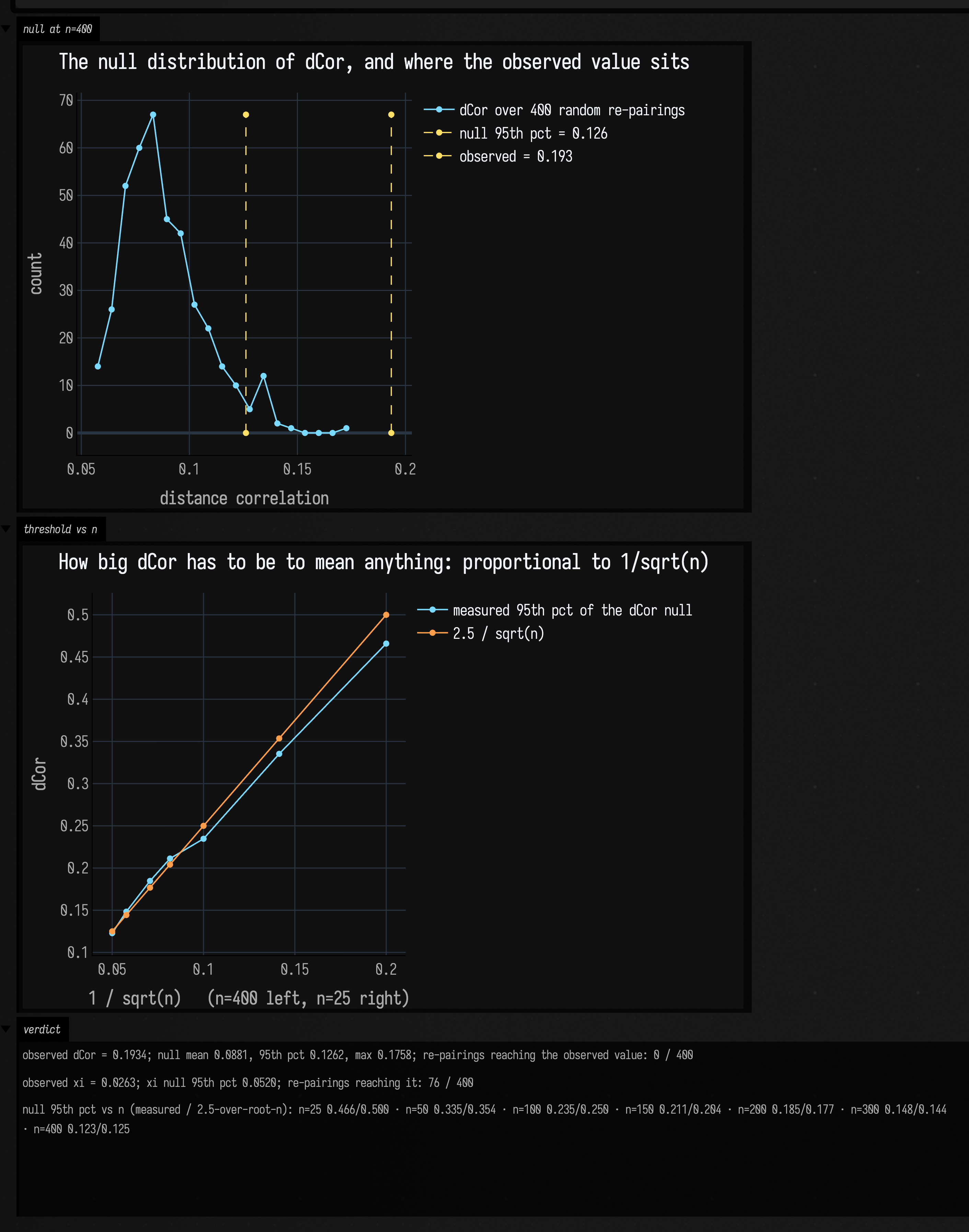
Read the verdict line. The observed 0.1934 is beyond every one of 400 random re-pairings
(0 / 400), whose 95th percentile is 0.1262 and whose maximum is 0.1758. The dependence is real
even though pearson reads −0.002. And in the same run xi reads 0.0263 against its own null's 95th
percentile of 0.0520, with 76 / 400 re-pairings doing at least as well: this run does not give strong evidence from xi.
The second figure gives you the shortcut for next time. Plotted against \( 1/\sqrt{n} \) rather than n, the
measured 95th percentile falls on a straight line through the origin, and the line's slope is
about 2.5. Read the measured-against-predicted pairs off the bottom of the figure: 0.335/0.354 at
n = 50 through 0.123/0.125 at n = 400, with the rule erring safely high at n = 25 (0.466 measured
against 0.500 predicted). For these independent Gaussian samples, \( 2.5/\sqrt{n} \) is a useful rough reference, not a universal
significance threshold. Measure the null for your own data. Note what the example means
for short signals. At n = 50 the threshold is around 0.34, so anything short of a strong
relationship is invisible; distance correlation needs a few hundred samples before it can see a
subtle one.
Rolling: finding when the relationship starts
A single coefficient over a whole recording answers the wrong question if the relationship comes
and goes. RollingDistanceCorrelation maintains its row sums, grand sums and cross sums
incrementally, so a push costs O(w) rather than the O(w²) a rebuild would
(correlations.kt:673). RollingXiCorrelation makes no such promise. It recomputes
chatterjeeXi over the window every time, at O(w log w) (correlations.kt:917–
correlations.kt:928). That makes it exactly as trustworthy as the batch call and no faster.
:::static
val w = 80
val total = 600
val change = 300
val rng = java.util.Random(3)

val dcor = RollingDistanceCorrelation(w)
val xiRoll = RollingXiCorrelation(w)

val xs = ArrayList<Double>()
val ys = ArrayList<Double>()
val dSeries = ArrayList<Double>()
val xiSeries = ArrayList<Double>()
val absR = ArrayList<Double>()

for (i in 0 until total) {
    val xv = rng.nextGaussian()
    // Before `change`: two independent Gaussians. After: y = x^2 - 1, a dependence Pearson cannot see.
    val yv = if (i < change) rng.nextGaussian() else xv * xv - 1.0 + 0.15 * rng.nextGaussian()
    xs += xv
    ys += yv
    val distanceValue = dcor.push(xv, yv)
    val xiValue = xiRoll.push(xv, yv)
    // Compare with the w-sample null only once a complete window has arrived.
    val fullWindow = xs.size >= w
    dSeries += if (fullWindow) requireNotNull(distanceValue) else Double.NaN
    xiSeries += if (fullWindow) requireNotNull(xiValue) else Double.NaN
    // There is no RollingPearson, so take the batch one over the same window for comparison.
    val lo = maxOf(0, xs.size - w)
    val bx = xs.subList(lo, xs.size).toDoubleArray()
    val by = ys.subList(lo, ys.size).toDoubleArray()
    absR += if (fullWindow) abs(StatsDependence.pearson(bx, by)) else Double.NaN
}

// Calibrate each statistic against its own null distribution at this window size.
// These are pointwise reference levels, not a multiple-testing-adjusted change detector.
val r2 = java.util.Random(1234)
val k = 300
val dNull = DoubleArray(k)
val xiNull = DoubleArray(k)
repeat(k) { i ->
    val nx = DoubleArray(w) { r2.nextGaussian() }
    val ny = DoubleArray(w) { r2.nextGaussian() }
    dNull[i] = StatsDependence.distanceCorrelation(nx, ny)
    xiNull[i] = StatsDependence.chatterjeeXi(nx, ny)
}
val threshold = dNull.sortedArray()[(k * 0.95).toInt()]
val xiThreshold = xiNull.sortedArray()[(k * 0.95).toInt()]

// The incremental sums are not an approximation. Cross-check the last window against the O(w^2)
// batch call, which materialises two full w x w distance matrices to get the same answer.
val batchLast = StatsDependence.distanceCorrelation(xs.takeLast(w).toDoubleArray(), ys.takeLast(w).toDoubleArray())
val agreement = abs(dSeries.last() - batchLast)

val firstD = (change until total).firstOrNull { dSeries[it] > threshold }
val firstXi = (change until total).firstOrNull { xiSeries[it] > xiThreshold }
val dCrossing = firstD?.let { "+${it - change} samples" } ?: "not crossed"
val xiCrossing = firstXi?.let { "+${it - change} samples" } ?: "not crossed"
:::fold the traces
showSignals(
    "rolling dCor" to dSeries,
    "rolling xi" to xiSeries,
    "rolling |pearson|" to absR,
    "dCor null 95th pct at w=$w" to List(total) { threshold },
    "xi null 95th pct at w=$w" to List(total) { xiThreshold },
    channel = "traces",
    title = "Three rolling coefficients across one regime change (window $w)",
    xTitle = "sample",
    yTitle = "coefficient",
    marks = ["regime change" to change],
)
// The two windows are the same three coefficients measured twice, so they read as a table.
// The pipes in `|r|` are escaped, or they would split the cell they sit in.
markdown(
    "numbers",
    """
    | window | dCor | xi | \|r\| |
    |--------|------|----|-------|
    | window-full to the change (i=$w..${change - 1}) | ${dSeries.subList(w, change).average().f3} | ${xiSeries.subList(w, change).average().f3} | ${absR.subList(w, change).average().f3} |
    | settled after the change (i=${change + w}..${total - 1}) | ${dSeries.subList(change + w, total).average().f3} | ${xiSeries.subList(change + w, total).average().f3} | ${absR.subList(change + w, total).average().f3} |

    {muted:dCor null 95th pct ${threshold.f3}: $dCrossing.
    xi null 95th pct ${xiThreshold.f3}: $xiCrossing.}

    {muted:incremental vs batch on the final window: |difference| = $agreement}
""",
    width = 900,
)
:::endfold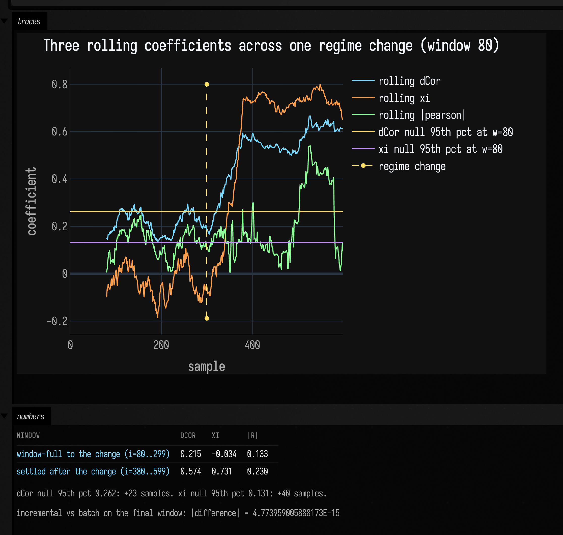
The measured numbers, from the run above:
| Measure | before the change | after it settles |
|---|---|---|
| rolling dCor | 0.215 | 0.574 |
| rolling xi | −0.034 | 0.731 |
| rolling |pearson| | 0.133 | 0.230 |
Each dependence measure is compared with its own null distribution at w=80. The
pointwise 95th-percentile levels describe independent Gaussian windows, and the figure reports
the first crossings for this seeded recording. Overlapping windows are correlated; these are
not multiple-testing-adjusted change alarms, and their first crossings do not establish a
general latency winner. Both settled dependence averages rise clearly after the change.
Rolling |pearson| still swings across much the same range before and after it: a small-window
absolute correlation has a positive noise floor, so reading it against zero would mislead.
The last line of that figure cross-checks two different algorithms.
RollingDistanceCorrelation never rebuilds a distance matrix (it only adds to and subtracts from
maintained sums), while StatsDependence.distanceCorrelation materialises two full w×w matrices
and double-centres them (correlations.kt:419–correlations.kt:499). On the final window they agree
to 5×10⁻¹⁵. The KDoc warns that the maintained sums accumulate floating-point drift over a
long run (correlations.kt:674),
and they do, though not far: over 200 000 pushes with a window of 64, the largest disagreement
sampled against the batch call was 8.6×10⁻¹⁴.
Agents: what pins the rolling bounds
RollingDependenceTest pins both bounds.
Reshaping a distribution: quantilewarp.kt
AdaptiveQuantileWarp does not measure anything: it fits a monotone 8-knot
PCHIP curve from the measured quantiles of recent samples onto the quantiles of a target
distribution, so a signal of the wrong shape becomes one of the right shape. The default target is
TargetDistributions.UnitNormal (quantilewarp.kt:94), and the default eight probabilities are
0.001, 0.01, 0.05, 0.20, 0.50, 0.80, 0.95, 0.99, which are not symmetric
(quantilewarp.kt:46), so the fit spends more knots on the left tail than the
right.
:::static
val rng = java.util.Random(5)
val fit = DoubleArray(4000) { exp(rng.nextGaussian()) } // log-normal: violently right-skewed
val held = DoubleArray(4000) { exp(rng.nextGaussian()) } // a second, disjoint draw

val warp = AdaptiveQuantileWarp() // target: UnitNormal, 8 knots
val state = warp.update(fit)

val warped = held.map { state.evaluate(it) }
val before = buildSummaryStats(held.toList())
val after = buildSummaryStats(warped)

/*
An independent oracle for the 8-knot fit: the *exact* warp onto a unit normal is
Phi^-1(Fhat(v)), the inverse normal CDF of the empirical CDF of the fitting sample. Nothing in
`quantilewarp.kt` computes that, so comparing against it tests the PCHIP interpolation itself.
*/
val sortedFit = fit.sortedArray()
fun empiricalCdf(v: Double): Double {
    var lo = 0
    var hi = sortedFit.size
    while (lo < hi) {
        val mid = (lo + hi) / 2
        if (sortedFit[mid] <= v) lo = mid + 1 else hi = mid
    }
    return lo / sortedFit.size.toDouble()
}

val probes = (2..98).map { it / 100.0 }
val inputs = probes.map { sortedFit[(it * (sortedFit.size - 1)).toInt()] }
val pchip = inputs.map { state.evaluate(it) }
val exact = inputs.map { inverseStandardNormalCdf(empiricalCdf(it).coerceIn(1e-4, 1.0 - 1e-4)) }
val worst = pchip.indices.maxOf { abs(pchip[it] - exact[it]) }
:::fold the curve and the two distributions
showSignals(
    "8-knot PCHIP warp" to pchip,
    "exact inverse-normal of the empirical CDF" to exact,
    x = probes,
    channel = "the fitted curve",
    title = "The warp, against the exact answer it is approximating",
    xTitle = "quantile of the fitting sample",
    yTitle = "warped value",
    width = 900,
    height = 300,
)
// The two curves above are too close to tell apart, so plot their difference.
showSignals(
    "PCHIP − exact" to pchip.indices.map { pchip[it] - exact[it] },
    x = probes,
    channel = "the error",
    title = "How far the 8-knot warp is from the exact one",
    xTitle = "quantile of the fitting sample",
    yTitle = "PCHIP − exact",
    // The knots inside the plotted range, where the error must be zero.
    marks = QuantileWarpConfig().probabilities.filter { it in 0.02..0.98 }.map { "knot at $it" to it },
    width = 900,
    height = 260,
)
val svgs = [
    histogramToSvg(
        buildHistogram(held.toList()),
        widthPx = 460,
        heightPx = 250,
        padTop = 26,
        decimals = 2,
        title = "held-out input: skew ${before.skewness.f1}",
    ),
    histogramToSvg(
        buildHistogram(warped),
        widthPx = 460,
        heightPx = 250,
        padTop = 26,
        decimals = 2,
        title = "after the warp: skew ${after.skewness.f3}",
    ),
]
showRow("distributions", svgs)
// before/after over the same four moments: a table says it in a quarter of the characters.
markdown(
    "numbers",
    """
    | held-out | mean | sd | skew | excess kurtosis |
    |----------|------|----|------|-----------------|
    | before | ${before.mean.f3} | ${before.sampleStdDev.f3} | ${before.skewness.f3} | ${before.kurtosisExcess.f1} |
    | after | ${after.mean.f4} | ${after.sampleStdDev.f4} | ${after.skewness.f4} | ${after.kurtosisExcess.f4} |

    {muted:input knots: ${state.inputKnots.joinToString { it.f3 }}}

    {muted:target knots: ${state.targetKnots.joinToString { it.f3 }}}

    {muted:worst |PCHIP - exact| over the 2nd..98th percentile: ${worst.f4}}
""",
    width = 900,
)
:::endfold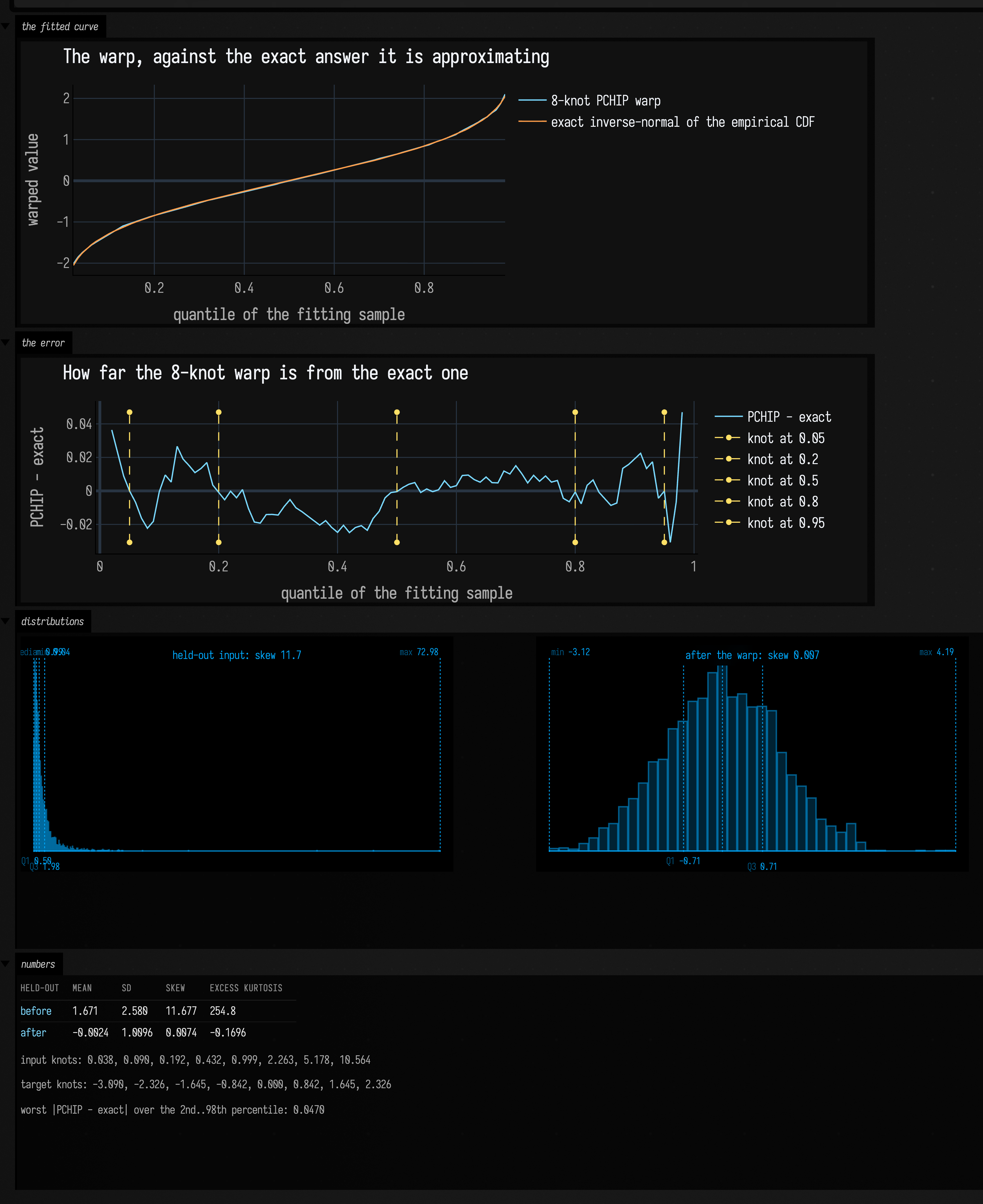
It works, and it works out of sample: the curve is fitted on fit and every number reported is
measured on the disjoint held. Skewness goes from 11.68 to 0.0074, excess kurtosis from
254.8 to −0.170, mean to −0.0024 and standard deviation to 1.0096. Eight knots and a PCHIP
is enough to turn a log-normal into something you can treat as normal, and the second plot says how
much is lost doing it: over the 2nd-to-98th percentile the 8-knot curve is within 0.047 of the
exact \( \Phi^{-1}(\hat{F}(v)) \) it is approximating. The left histogram in the same figure is the reason you
would bother: with a maximum of 72.98 against a median of 0.98, the raw distribution is one spike
and a tail, and no amount of binning makes it readable. Nothing in quantilewarp.kt computes that
exact answer, so the oracle is built in the fence out of inverseStandardNormalCdf
(quantilewarp.kt:908, itself accurate to six decimals: it returns 1.959964 at p=0.975 and
−3.090232 at p=0.001) and a binary search over the sorted fitting sample.
Three things to watch for:
- Outside the fitted range,
evaluateextrapolates linearly from the endpoint tangent (quantilewarp.kt:183), and for a compressed tail that slope is steep. On the fit above, whose lowest input knot is 0.038,evaluate(0.0)returns −3.75 andevaluate(-1.0)returns −21.1. Nothing clamps it. If your signal can leave the range you fitted on, clamp the input yourself. - Successive states are smoothed, not replaced.
smoothingAlphadefaults to 0.20 (quantilewarp.kt:146) and eachupdatelerps the previous knots 20% of the way to the new ones (quantilewarp.kt:357). Feed a signal whose median jumps from 0 to 10 and the median knot goes 0.009 → 2.016 → 3.608 → 4.879 → … → 9.310 after twelve updates, tracking \( 10\cdot(1 - 0.20)^k \): 0.690 remaining against a predicted 0.687. Convergence is geometric, so a step change takes a couple of dozen frames to follow. - The knots are forced strictly increasing after smoothing
(
quantilewarp.kt:364), so the curve stays invertible even when the input degenerates; swept from −5 to 60 in steps of 0.01 the fitted curve above is strictly increasing throughout.
AdaptiveQuantileWarp also keeps a history: update merges the batch you hand it with the last
historyFrames batches (default 8, quantilewarp.kt:139) before
taking quantiles, so the knots are fitted on eight frames' worth of samples, not one. And the whole
state packs into four vec4s for push constants. applyToPushConstants plus the matching GLSL
include named by FIELD_QUANTILE_WARP_INCLUDE_NAME evaluate the identical curve on the GPU, and
Box.fieldProbeQuantileWarp (quantilewarp.kt:553) closes that
loop for you: it installs a runloop hook that drains a shader field probe,
updates the warp and calls your apply callback with the new state.
Choosing, in one paragraph
Start with distanceCorrelation as one screen for dependence. Its population value is zero under
independence, but finite samples have a noise floor: estimate that floor for your data, for example
with the permutation test above. If it fires, ask what shape: pearson
for a line, spearman or kendallTauB for monotone-but-curved, xi for "is y a function of
x" including non-monotone ones. Hand xi its two arrays in the order you mean them, since it is
the one coefficient here that answers a different question when you swap them. Reach for
micTicNaive only for intuition, and never to compare against published MIC numbers. Above a few
thousand samples, kendallTauB and distanceCorrelation are both O(n²) and distanceCorrelation
also allocates two n×n matrices, so switch to RollingDistanceCorrelation or subsample. And if the
problem turns out to be that the signal is the wrong shape rather than unrelated to anything, that
is quantilewarp.kt.
Everything on this page is also available as live, editable boxes: the statistics_examples starting
point listed under Pure-compute scenes in
Agent transcripts opens the whole thing in a fresh
document, each box printing the numbers above so a re-run checks itself. Change a shape, a window
size, a target distribution or an n and re-run one.
For the signals themselves rather than these derived quantities, see the time-domain signal examples; for recovering a hidden state from noisy measurements, State estimation; and for the rolling-dependence fences in their original setting, Values Over Time. For a distribution over whole functions, curves and fields — means, uncertainty and coherent draws from a few observations — see Drawing with Gaussian processes.
The public declarations used on this page are listed, with their KDoc, in the codebase reference: Math and Data.