Field 4 Graphics
Build a window, draw into it, and then start changing what the GPU does. This curriculum takes you from a triangle through cameras, textures, compute shaders and particles, with each lesson in a box you can run and edit. For a shorter first encounter, try Graphics on the GPU.
Open Welcome → Starting points → canonical_graphics to get an editable copy of this complete graphics curriculum, including its code and shader sidecars. Launch the window box first, then the lesson you want to explore. The bundled original stays unchanged, and opening it again makes another fresh copy.
Field 4 is Field's direct Vulkan path. Vulkan is a powerful, low-level graphics API that is notorious for how hard it is to write code for. Field turns it into something that is pleasant to hack on in real time. But p5.js it ain't.
A graphics box usually has three parts:
- Kotlin code that creates modules, meshes, buffers, cameras, textures, and renderer connections.
- Shader properties: properties of the box, such as
vertex,fragment,compute, orvertex_fragment, that hold GLSL code. You switch the code editor to one of them and edit it like the box's Kotlin. - Reflected accessors that Field generates by reading the shader interface. Field compiles the shaders, reads which inputs, buffers, uniforms and push constants they declare, and gives the box Kotlin properties with the same names, so you never write binding numbers or byte offsets by hand.
In any graphics engine, the low-level view that the GPU has of the data and the high-level CPU view of it have to match. In Field the low-level view is written in GLSL (or Slang), and the high-level view in Kotlin (or another of Field's languages). The GLSL drives that conversation, and the Kotlin side follows it. If a vertex shader declares layout(location = 0) in vec3 pos, the Kotlin side can write pos.add(...) inside m.set { ... }. If a shader declares a push constant member named vertexData, the Kotlin side can assign m.vertexData = { vertexData }. A shader is both the code that runs on the GPU and the contract that shapes the Kotlin API for its box.
This page is about the low-level Vulkan pieces: what you need for the kind of shader hacking
behind a lot of new media art and data visualization. For more standard photorealistic rendering,
progressive PBR with environment lighting, glass and editable
material shaders, see Progressive path tracing, including
glTF and GLB import. It renders into
an ordinary RenderToTexture, so its output can be combined with the techniques
in this guide. The firefly controls help
keep interactive previews clean.
Hello triangle, first attempt
Start with the rite of passage for any new graphics system: getting a triangle on the screen. That needs one of everything: one shader module, one mesh to draw, one renderer and one window. moduleHere { ... } creates a shader module from the current box's shader properties. Mesh() creates draw data. module += m named "my mesh" attaches the mesh to the module, and renderer += module makes the module part of the window.
// A module is one draw pipeline: this box's `vertex` and `fragment` shaders plus
// the meshes it draws. `renderer` is inherited from the renderer parent box.
var module = moduleHere {
    primitiveType = triangle_strip
}

// A Mesh holds vertex buffers whose names come from the vertex shader's `in`
// attributes (`pos`, `col`), plus the index buffer `tri`.
var m = Mesh()
module += m named "my mesh"
renderer += module

// Room for 3 vertices and 3 indices; inside, `pos`, `col` and `tri` append data.
m.set(3, 3) {
    // x, y, z for each of the three corners, in clip space (-1..1)
    pos.add(0, 0, 0, 0.5, 0, 0, 0.5, 0.5, 0)

    // one RGBA colour per vertex, `it` running 0, 1, 2
    3 {
        col.add(0, it / 3.0, 1 - it / 3.0, 1)
    }
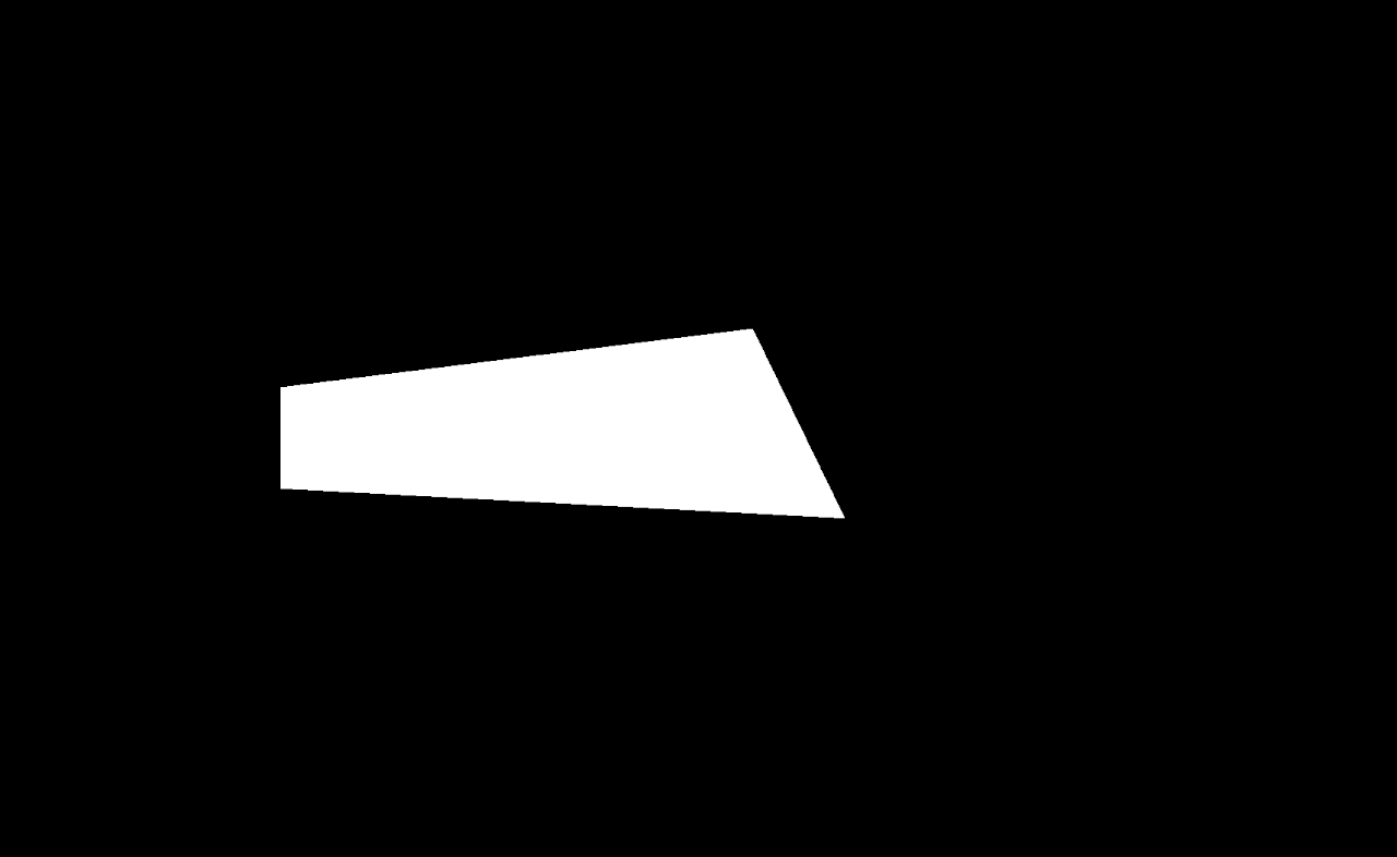
    tri.add(0, 1, 2)
}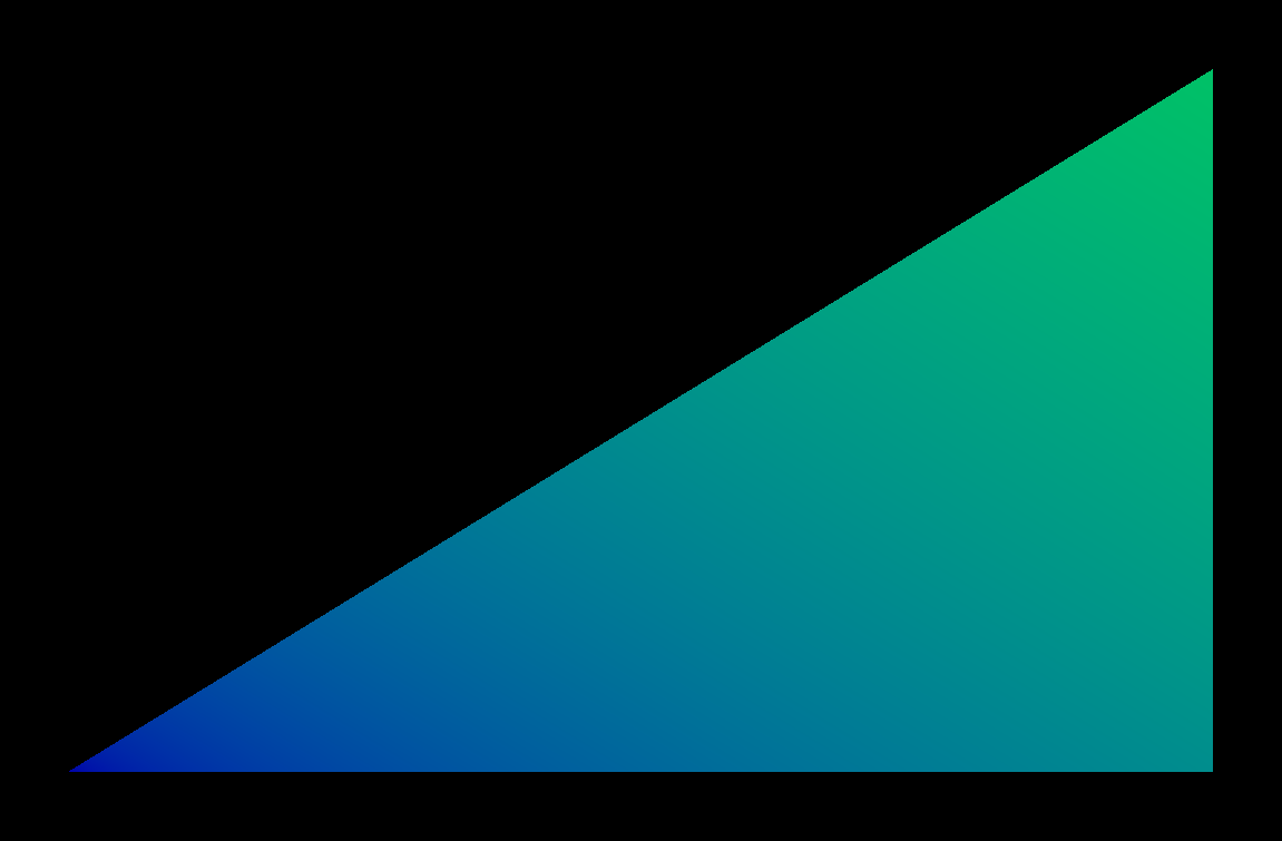
The m.set(3, 3) call says: allocate three vertices and three indices. Inside that block, pos, col, and tri are generated writers. tri.add(0,1,2) gives the triangle strip its three indices.
The vertex shader declares the attributes that produce those generated writers:
#version 450
layout (location = 0) in vec3 pos;
layout (location = 1) in vec4 col;
layout (location = 0) out vec4 fcol;

void main()
{
    fcol = col;
    gl_Position = vec4(pos, 1);
}
layout(location = 0) in vec3 pos is why Kotlin can compile something like pos.add(...). layout(location = 1) in vec4 col is why Kotlin can compile col.add(...). The shader copies col to fcol, and the fragment shader receives that value at the matching location:
#version 450
layout(location = 0) out vec4 uFragColor;
layout(location = 0) in vec4 fcol;

void main()
{
    uFragColor = vec4(1.0, 0.8, 0.4, 1.0) * fcol;
}
The first example is as small as it can be: vertex data is written directly into the mesh, the shader reads it as vertex attributes, and the fragment shader colors the pixels.
Hello triangle, second attempt
The first triangle put pos and col directly into the mesh's vertex buffers. That is completely supported, and it is the closest to what you were taught if you learned OpenGL (or Three.js), but it is not the most general or flexible way to feed a shader. Sometimes you want a buffer that is visible as an ordinary named resource in the shader: perhaps the geometry changes every frame, perhaps a compute shader fills it, or perhaps several draws share it. This example uses the simplest version of that pattern: write a few positions into a defaultBuffer, bind that buffer to a reflected push-constant member, and draw vertices by index.
var module = moduleHere { primitiveType = triangles }
var m = Mesh()
module += m named "someMesh"
renderer += module

var vertexData = defaultBuffer {
    perFrame = true
    size = 9.vec4s
}
    .buffer

m.vertexData = { vertexData }

vertexData.write {
    put(vec(-0.8, -0.6, 0.0, 1.0))
    put(vec(-0.2, -0.6, 0.0, 1.0))
    put(vec(-0.5, 0.2, 0.0, 1.0))

    put(vec(-0.1, -0.4, 0.0, 1.0))
    put(vec(0.5, -0.4, 0.0, 1.0))
    put(vec(0.2, 0.5, 0.0, 1.0))

    put(vec(0.2, -0.8, 0.0, 1.0))
    put(vec(0.8, -0.8, 0.0, 1.0))
    put(vec(0.5, 0.0, 0.0, 1.0))
}

m.resize(9)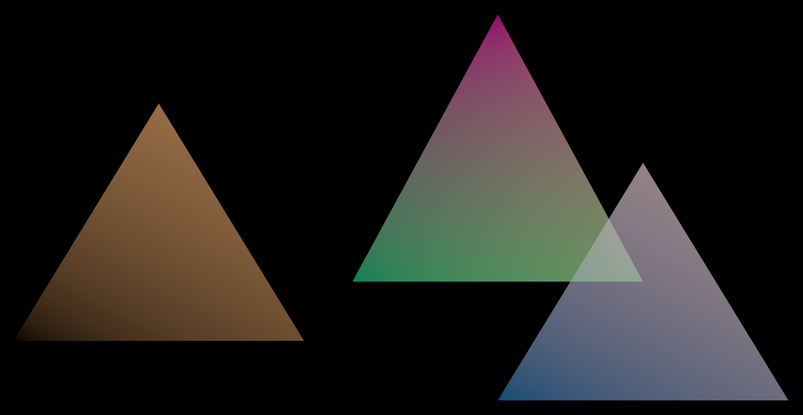
There are three moving pieces here. defaultBuffer { ... }.buffer allocates GPU-visible storage. vertexData.write { ... } fills it with nine vec4 positions, three per triangle. m.resize(9) tells the draw to consume nine vertices. If this were animated, the same code would move the write and resize calls into a frames { ... } loop (see Frames and the animation loop).
The shader side uses a Vulkan buffer reference:
#version 450
#extension GL_EXT_buffer_reference : require

layout(std430, buffer_reference) buffer vertexData
{
    vec4 positions[];
};

layout(push_constant) uniform matrices {
    mat4 p;
    mat4 m;
    vertexData vertexData;
} pc;

layout(location=0) out vec4 localColor;

float wrap(int a, int b) {
    // Divide as floats so the ramp includes intermediate channel values.
    return float(a % b) / float(b - 1);
}

void main()
{
    gl_Position = vec4(pc.vertexData.positions[gl_VertexIndex].xyz, 1);
    localColor = vec4(
    wrap(gl_VertexIndex, 3),
    wrap(gl_VertexIndex, 5),
    wrap(gl_VertexIndex, 11),
    1.0);
}
The important name is vertexData. It appears in the push constant block, so Field reflects it into m.vertexData. The Kotlin line m.vertexData = { vertexData } binds the buffer created in Kotlin to the shader member read as pc.vertexData.
The fragment shader just consumes the color produced by the vertex shader:
#version 450
layout(location = 0) out vec4 uFragColor;
layout(location = 0) in vec4 localColor;

void main()
{
    uFragColor = vec4(localColor.rgb, 0.3);
}
Camera matrices in a UBO
The previous two examples draw in clip-space coordinates. To draw from a camera, the shader needs projection and view matrices. This version stores those matrices in a uniform buffer owned by the module.
var m = Mesh()
var module = moduleHere()

module += "mainMesh" to m
renderer += module

val camera = Camera()
camera.at = vec(-8, 2, 7)

module.view.m = camera.m()
module.view.p = camera.p()

for (n in 1..80) {
    m.set(3 * n, 1 * n) {
        n {
            val z = 0.0 + it
            pos.add(0, 0, -1 + z, 1.0, 0.1, z, 1, 1, z)
            3 {
                col.add(10 - it * 0, it / 3.0, 1 - it / 3.0, 1)
            }
            tri.add(0 + 3 * it, 1 + 3 * it, 2 + 3 * it)
        }
    }
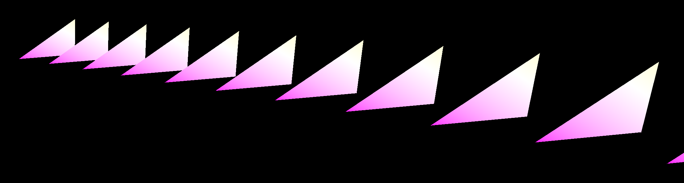
}
The shader declares a UBO named view:
#version 450
layout (location = 0) in vec3 pos;
layout (location = 1) in vec4 col;
layout (location = 0) out vec4 fcol;

layout (set=0, binding = 0) uniform view {
    mat4 p;
    mat4 m;
} cam;

void main()
{
    gl_Position = cam.p * cam.m * vec4(pos, 1);
    fcol = col;
}
Because the uniform block is named view, the Kotlin side writes module.view.p and module.view.m. The module owns this resource because the block is declared at descriptor set/binding scope, not as a per-mesh push constant.
moduleHere() generates a Kotlin class per uniform block, named by capitalising the block's name. When that name is already a type the box imports, the class gets Block on the end instead: a block called camera generates CameraBlock, so Camera() is still Field's camera.
Camera as push constants
For quick sketches, it is often simpler for the mesh to carry the camera matrices as push constants. The draw data still lives in m, but now m.p and m.m are assigned directly before the draw.
var m = Mesh()
var module = moduleHere()

module += "mainMesh" to m
renderer += "boo" to module

val camera = Camera()
camera.at = vec(-8, 2, 7)

m.p = camera.p
m.m = camera.m

for (n in 1..80) {
    m.set(3 * n, 1 * n) {
        n {
            val z = 0.0 + it
            pos.add(0, 0, -1 + z, 1.0, 0.1, z, 1, 1, z)
            3 {
                col.add(0, it / 3.0, 1 - it / 3.0, 1)
            }
            tri.add(0 + 3 * it, 1 + 3 * it, 2 + 3 * it)
        }
    }
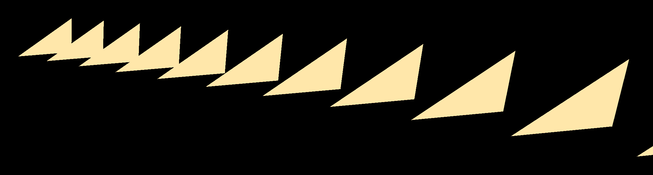
}
The GLSL is almost identical to the UBO version, but the matrices are now push constants:
#version 450
layout (location = 0) in vec3 pos;
layout (location = 1) in vec4 col;
layout (location = 0) out vec4 fcol;

layout(push_constant) uniform matrices {
    mat4 p;
    mat4 m;
} pc;

void main()
{
    gl_Position = pc.p * pc.m * vec4(pos, 1);
    fcol = col;
}
That is why the Kotlin changed from module.camera.p = ... to m.p = .... p and m are reflected onto the mesh because the shader reads them from the per-draw push constant block.
Keyboard camera
KeyCamera does not change the shader contract. It wraps a Camera and updates it from keyboard input while the renderer runs.
var module = moduleHere()
var m = Mesh()

module += m named "mainMesh"
renderer += module

val camera = Camera()
// The quad runs from (0, 0) to (1, 1): aim at its centre, close enough that it fills the window.
camera.at = vec(0.5, 0.5, -0.8)
camera.target = vec(0.5, 0.5, 0)
m.p = camera.p
m.m = camera.m

m.set(3, 1) {
    val z = 0.0
    pos.add(0, 0, 0 + z, 1.0, 0.1, z, 1, 1, z)
    tri.add(0, 1, 2)
}

var kc by keyCamera(camera = camera)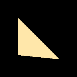
The shader is the same push-constant shape as the previous section, just without the color attribute. Camera control is ordinary Kotlin state around the same rendering contract.
With the render window focused, these keys move the camera. Movement glides to a stop after you let go, and steps are a fraction of the distance to the camera's target, so the same key moves less up close.
| Key | Moves | With Shift |
|---|---|---|
| W / Up, S / Down | forward, back (the target moves too) | forward, back toward a fixed target |
| A, D | left, right | the same, with the target fixed |
| E, C | up, down | the same, with the target fixed |
| Left, Right | turn in place | orbit around the target |
| Page Up, Page Down | tilt in place | orbit up and down around the target |
Z / ,, X / . |
roll | |
-, = |
narrow, widen the field of view | in finer steps |
| R | reset to where the camera started |
Re-running the box replaces the controls rather than adding a second set, because keyCamera registers them under the property's name (kc here).
Compute shader
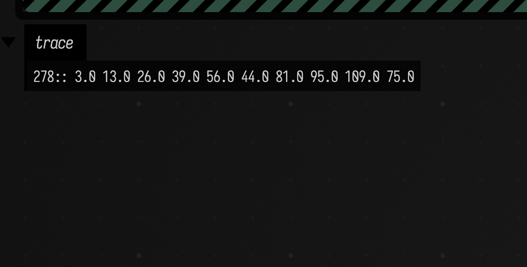
Compute modules use the same box model, but instead of drawing vertices they dispatch workgroups: groups of GPU threads that run the same shader together. This example writes an input buffer, dispatches a ComputeMesh, reads the output buffer back every frame, and shows the first ten floats in the box's trace output channel. Nothing is drawn to the graphics window; the trace is the result:
var numVec4 = 16

var module = computeModuleHere {
    ssboSizer = { ubo ->
        numVec4 * 4 * 4
    }
}

var m = ComputeMesh()
var localSize = 16
// Include a partial final group; the shader guards both buffer lengths.
m.x = (numVec4 + localSize - 1) / localSize
m.y = 1
m.z = 1

module += "mainInvocation" to m
renderer += "runCompute" to module

module.InputBuffer.mapAndWrite {
    this.clear()
    for (n in 0 until numVec4) {
        this.add(n.toFloat() * 13.0)
    }
    this.clear()
}

var fr = 0
frames {
    while (true) {
        module.OutputBuffer.mapAndRead {
            var s = "${fr}:: "
            this.clear()
            for (n in 0 until 10) s += this.get(n).toString() + " "
            display("trace", s)
        }

        fr++
        frame()
    }
}
The compute shader declares its workgroup size and two storage buffers:
#version 450
layout(local_size_x = 16, local_size_y = 1, local_size_z = 1) in;

layout(set=0, binding = 0) writeonly buffer OutputBuffer {
    vec4 outData[];
};

layout(set=0, binding = 1) readonly buffer InputBuffer {
    vec4 inData[];
};


void main() {
    uint idx = gl_GlobalInvocationID.x;
    // Array lengths reflect the actual SSBO allocation, including edited element counts.
    if (idx >= uint(min(inData.length(), outData.length()))) return;
    outData[idx] = inData[idx] * vec4(1,1,1,1) +
    vec4(3 + idx * 1, -(idx * 21.0), idx * 3, idx * 4);
}
layout(local_size_x = 16) matches the Kotlin localSize. m.x, m.y, and m.z set the dispatch dimensions, counted in workgroups. Here numVec4 is 16 and localSize is 16, so m.x = (16 + 16 - 1) / 16 = 1: one workgroup of 16 × 1 × 1 threads, 16 invocations in all, one per vec4. With numVec4 = 20 it would be two workgroups, 32 invocations, and the idx >= guard in the shader stops the 12 that have no element. The storage-buffer names become module.InputBuffer and module.OutputBuffer, which is why Kotlin can map and read/write them directly.
Compute particles, then draw them
The compute example above dispatched a shader and read the result back on the CPU. The more useful pattern keeps the data on the GPU: one box computes into a buffer, a second box draws from that same buffer, and the two are wired together through the box graph rather than through a shared global.
This is the first example that needs two boxes, so it is also the first place the graph topology matters: the draw box is connected beneath the compute box, which publishes its output buffer as a property:
fieldProbeHere(1000).display("probe")
displayOpen("probe")

var module = computeModuleHere {}
var m = ComputeMesh()

module += "mainMesh" to m
renderer += "module" to module

// N changes buffer allocation. Stop the draw child first; rerun compute, then draw.
val N = 100000
var inData = defaultBuffer { size = N.vec4s }.buffer
var outData = defaultBuffer { size = N.vec4s }.buffer

m.inData = { inData }
m.outData = { outData }

var x = 0.0
m.something = {
    x += 0.01
    x.f
}

prop<FrameBufferGroup>(outputPositions) = outData
prop<Int>(particleCount) = N

// uint push members accept Int lambdas; the shader checks the tail group.
m.count = { N }

m.x = (N + 63) / 64
m.y = 1
m.z = 1

inData.write {
    for (x in 0 until N) {
        put(vec(Math.random(), Math.random(), Math.random(), Math.random()))
    }
}
The two prop<…> lines are the publication: outputPositions is the buffer and particleCount is how many particles it holds, and any box beneath this one inherits both. The dispatch is (N + 63) / 64 groups of 64, rounded up so no particle is left out; the extra lanes in the last group are why m.count = { N } passes the count to the shader, which returns early for any index at or past it. Because N sets the buffer sizes, changing it is a rebuild rather than a live edit: stop the draw child first, so it is not reading a buffer that is about to be replaced, then rerun this box and then the draw box. m.something = { ... } is a reflected push-constant member fed by a Kotlin lambda re-evaluated every dispatch, which is how the animation clock reaches the shader.
The compute shader takes both buffers as buffer references through its push-constant block, and calls fieldProbe to sample a value for the probe display:
#version 450
#extension GL_EXT_buffer_reference : require
layout(local_size_x = 64) in;

layout(std430, buffer_reference) buffer inData {
    vec4 a[];
};
layout(std430, buffer_reference) buffer outData {
    vec4 a[];
};

{% property "fieldProbe" %}

layout(push_constant) uniform dat {
    inData inData;
    outData outData;
    float something;
    uint count;
} pc;

void main() {
    uint idx = gl_GlobalInvocationID.x;
    // Ceiling dispatch includes extra lanes; none may access the particle buffers.
    if (idx >= pc.count) return;
    pc.outData.a[idx].x = pc.inData.a[idx].x*cos(pc.something*pc.inData.a[idx].z) + pc.inData.a[idx].y*sin(pc.something*pc.inData.a[idx].w);
    pc.outData.a[idx].y = -pc.inData.a[idx].x*sin(pc.something*pc.inData.a[idx].w) + pc.inData.a[idx].y*cos(pc.something*pc.inData.a[idx].z*0.03);

    fieldProbe(pc.outData.a[idx].y);

    pc.outData.a[idx].zw = pc.inData.a[idx].zw;
}
{% property "fieldProbe" %} is Field's shader templating pulling in the probe preamble; see Field probes. Templating in general is Shader templating below.
The draw box is a child of the compute box, and that is the only reason outputPositions resolves:
var module = moduleHere {
    primitiveType = triangles
}

var m = Mesh()

module += "mainMesh" to m
renderer += "boo2" to module

m.inData = { outputPositions }

// Inherit the count from the same parent that owns the buffers.
val N = particleCount

m.aspectRatio = { window.width / window.height.toFloat() }
m.set(N * 2 * 3, 0) {}

m
m.inData = { outputPositions } reads the parent's published property by name and binds it to this shader's inData buffer reference, and particleCount comes from the same parent, so the draw always sizes itself to the buffer it reads. No buffer is copied and nothing round-trips through the CPU: both boxes point at the same GPU allocation. m.set(N*2*3, 0) {} allocates six vertices per particle with an empty writer block, because the vertex shader synthesizes each quad's corners from gl_VertexIndex instead of reading vertex attributes:
#version 450
#extension GL_EXT_buffer_reference : require

layout(std430, buffer_reference) buffer inData {
    vec4 pos[];
};

layout(location = 0) out vec2 tc;

layout(push_constant) uniform push {
    inData inData;
    float aspectRatio;
} pc;

const vec3[6] part = {
    vec3(0,0,0), vec3(1,0,0), vec3(1,1,0),
    vec3(0,0,0), vec3(1,1,0), vec3(0,1,0)
};

void main()
{
    float scale = 1.0 * pc.inData.pos[gl_VertexIndex/6].w;
    vec3 p = (part[gl_VertexIndex%6]-vec3(0.5, 0.5, 0))*scale;

    p.xy += pc.inData.pos[gl_VertexIndex/6].xy*10.0;
    p.xy *= vec2(1/pc.aspectRatio, 1);
    gl_Position = vec4(p*0.04, 1);

    tc = part[gl_VertexIndex%6].xy;
}
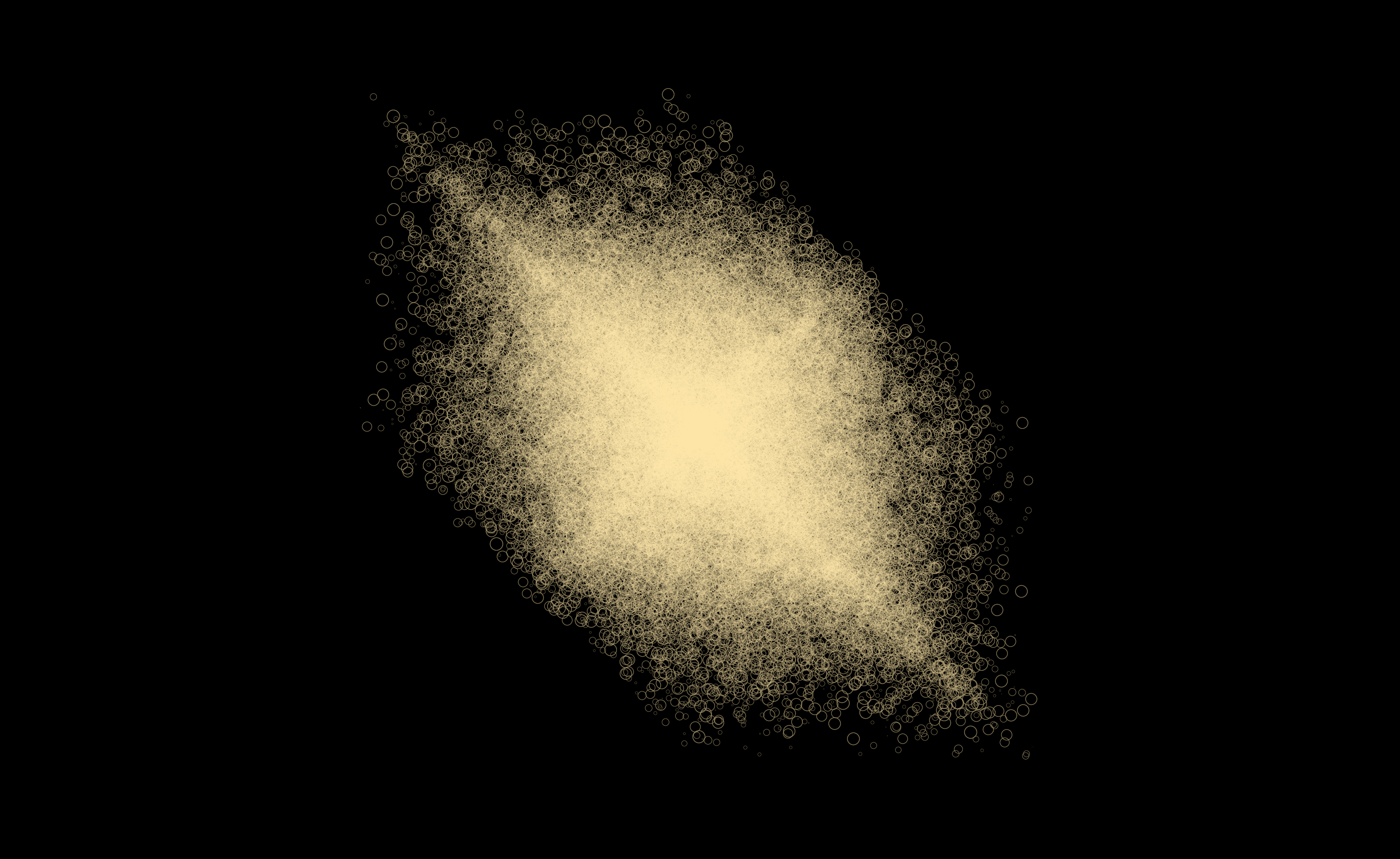
gl_VertexIndex / 6 picks the particle and gl_VertexIndex % 6 picks the corner: 100,000 particles drawn as 600,000 vertices with no index buffer and no per-particle CPU work.
Here are the three boxes on the canvas, renderer above compute above draw, each joined to the one beneath it:
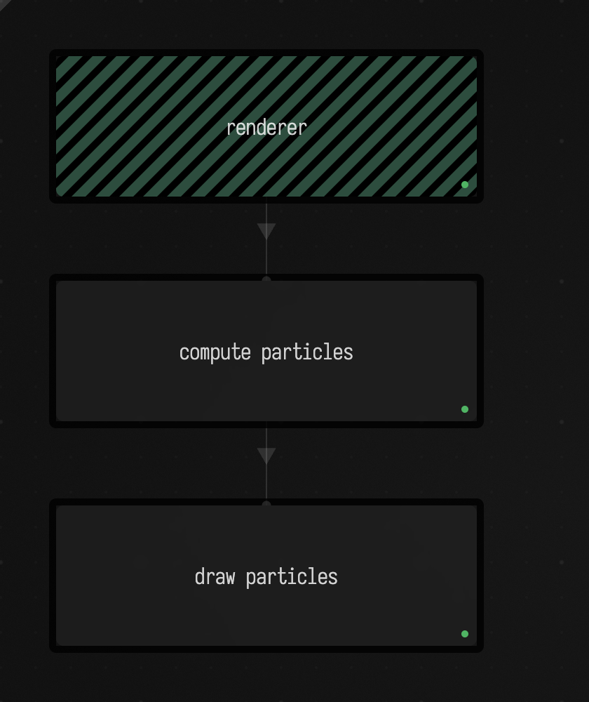
and what the draw box puts in the window: 100,000 particles drawn straight from the compute box's buffer.
To see it running, open the corpus document in the viewer above, or open threebox, the same renderer/compute/draw shape built as a runnable three-box scene.
Texturing
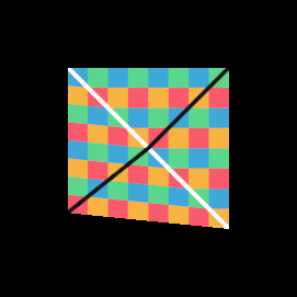
Textures add another reflected resource. The shader declares a sampler named bbc; Kotlin creates a LoadedTexture property with the same name and transfers it before drawing.
prop<LoadedTexture>(bbc) = LoadedTexture("public/docs/assets/afield_four_graphics/docs-checker-texture.png")
bbc.transferNow()

var module = moduleHere {}
var m = Mesh()

module += "mainMesh" to m
renderer += "boo" to module

val camera = Camera()
// The quad runs from (0, 0) to (1, 1): aim at its centre, close enough that it fills the window.
camera.at = vec(0.5, 0.5, -0.8)
camera.target = vec(0.5, 0.5, 0)
m.p = camera.p
m.m = camera.m

var kc by keyCamera(camera = camera)
m.set(4, 2) {
    val z = 0.0

    pos.add(0, 0, 0 + z, 1.0, 0.1, z, 1, 1, z, 0, 1, z)
    tc.add(0, 0, 1, 0, 1, 1, 0, 1)

    tri.add(0, 1, 2)
    tri.add(0, 2, 3)
}
The vertex shader now has two attributes: position and texture coordinate.
#version 450
layout (location = 0) in vec3 pos;
layout (location = 1) in vec2 tc;
layout (location = 1) out vec2 ftc;

layout(push_constant) uniform matrices {
    mat4 p;
    mat4 m;
} pc;

void main()
{
    gl_Position = pc.p * pc.m * vec4(pos, 1);
    ftc = tc;
}
layout(location = 1) in vec2 tc is why Kotlin has tc.add(...). The fragment shader receives ftc and samples the texture:
#version 450
layout(location = 0) out vec4 uFragColor;
layout(location = 1) in vec2 ftc;

layout(set = 0, binding = 0) uniform sampler2D bbc;

void main()
{
    vec4 c = texture(bbc, ftc.yx);
    uFragColor = vec4(c.rgb, 1.0);
}
The name bbc is the bridge. Kotlin creates prop<LoadedTexture>(bbc), the shader declares sampler2D bbc, and Field binds the texture resource by matching that reflected name.
Multi-texture
A shader can declare an array of samplers, and the Kotlin side binds it by publishing an array of image views under the array's name. The reflected-name contract is the same as the single texture above; only the type changes.
var bbc = LoadedTexture("public/docs/assets/afield_four_graphics/docs-checker-texture.png")
bbc.transferNow()

var bbc2 = LoadedTexture("public/docs/assets/rt-uv-gradient.png")
bbc2.transferNow()

var bbc3 = LoadedTexture("public/docs/assets/afield_four_graphics/spiral-texture.png")
bbc3.transferNow()

var asArray: Array<ImageView> = arrayOf(bbc.imageView, bbc2.imageView, bbc3.imageView)

prop<Array<ImageView>>(ta) = asArray

var module = moduleHere {}
var m = Mesh()

module += "mainMesh" to m
renderer += "boo" to module

val camera = Camera()
// The quad runs from (0, 0) to (1, 1): aim at its centre, close enough that it fills the window.
camera.at = vec(0.5, 0.5, -0.8)
camera.target = vec(0.5, 0.5, 0)
m.p = camera.p
m.m = camera.m

var kc by keyCamera(camera = camera)
m.set(4, 2) {
    val z = 0.0

    // four corners of the unit square, and the texture coordinate at each
    pos.add(0, 0, z)
    pos.add(1, 0, z)
    pos.add(1, 1, z)
    pos.add(0, 1, z)
    tc.add(0, 0, 1, 0, 1, 1, 0, 1)

    tri.add(0, 1, 2)
    tri.add(0, 2, 3)
}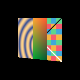
prop<Array<ImageView>>(ta) is the whole difference. Note that LoadedTexture is not itself the bindable resource; bbc.imageView is, which is why the array is built from image views rather than from the textures. Each entry here is a different image, the checkerboard, a colour gradient and a frame of the spiral from Graphics on the GPU, and the fragment shader picks one for each third of the quad.
The fragment shader declares the array and indexes it:
#version 450
layout(location = 0) out vec4 uFragColor;
layout(location = 1) in vec2 ftc;

layout(set = 0, binding = 0) uniform sampler2D ta[3];

void main()
{
    // Each third of the quad, left to right, shows one entry of the array. Every entry is sampled and the
    // result chosen afterwards, so the array index stays a constant.
    // ftc.yx swaps the texture coordinates, which transposes the image on the quad.
    vec4 c0 = texture(ta[0], ftc.yx);
    vec4 c1 = texture(ta[1], ftc.yx);
    vec4 c2 = texture(ta[2], ftc.yx);
    vec4 c = ftc.x < 1.0 / 3.0 ? c0 : (ftc.x < 2.0 / 3.0 ? c1 : c2);
    uFragColor = vec4(c.rgb, 1.0);
}
The declared array length (ta[3]) is the descriptor count, and the count must match exactly: publishing two views against ta[3] is refused at link time with can't link texture resource ta of length 2 but the shader expects 3, and the box draws nothing.
Loading a glTF model
Everything so far built its geometry in Kotlin. gltfModelHere(path) instead reads a glTF file and hands back a module and the meshes it found, with shaders written to match how that file lays out its data. Here it loads the Khronos toy car the Fabricate renderer pages use:
var (module, meshes) = gltfModelHere("public/docs/assets/fabricate_demo/ToyCar.glb")

var m = Mesh()
module += "car" to m
renderer += "boo" to module

// orthoness blends between perspective (0) and orthographic (1) projection.
val camera = Camera()
camera.p.orthoness = 0.3
camera.p.matchDepth = 2.0
camera.target = vec(0, 0.4, 0)
camera.at = vec(-2.2, 1.8, 2.9)

// Keyboard controls for the camera; R resets it.
KeyCamera(camera = camera)

/*
The file stands the car up and scales it to centimetres (a 0.0001 node scale); this model matrix
keeps the rotation and makes it about four units long. meshes[model].meshes[primitive]: copy
primitive 0 of model 0 into our mesh.
*/
val model = Matrix4f().rotateX(Math.PI.toFloat() / 2).scale(0.01f)
meshes[0].meshes[0].applyToMesh(m, camera, model)
camera.p()

loop {
    frame()
}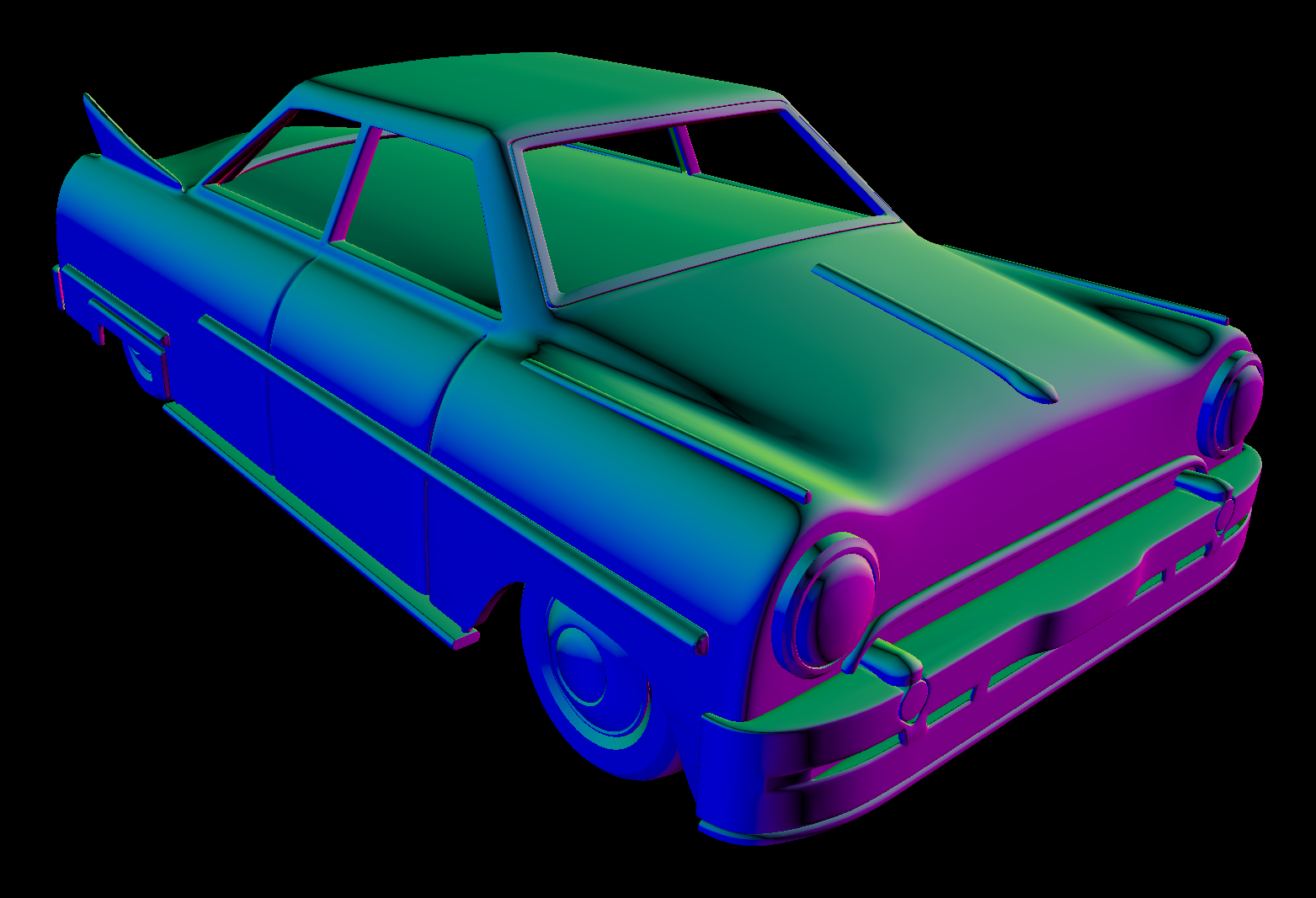
The colours are the written fragment shader's: it shades by the view-space normal, so faces turned the same way share a colour.
Three things to notice. meshes[0].meshes[0].applyToMesh(m, camera, model) copies one primitive of one model into your mesh; the outer index is the model, the inner one the primitive, so a multi-part file is addressed rather than flattened. The model matrix is there because this file stands the car up and scales it to a few centimetres with its own node transform: the box keeps the rotation and makes the car about four units long, a size the camera can frame. And camera.p.orthoness / camera.p.matchDepth are Field's blend between perspective and orthographic rather than a choice between them.
applyToMesh also fills the shader's modelView (view times model) and proj push constants from the camera every frame, which is why the loop has nothing to do but frame(). Geometry from disk has the measurement behind the composition.
The vertex shader shows what "matched to the data" means. Rather than declaring vertex attributes, it reads a flat float array through a buffer reference and unpacks by stride:
layout(std430, buffer_reference) readonly buffer VertexBuffer {
    float vertexData[];
};

layout(std430, buffer_reference) readonly buffer IndexBuffer {
    uint indexData[];
};

layout(push_constant) uniform PushConstants {
    mat4 modelView;        // view * model
    mat4 proj;             // projection
    vec4 materialBaseColor;
    uint vertexOffset;     // in floats
    uint indexOffset;      // in indices
    uint vertexStride;     // in floats
    uint useVertexColor;   // bool as uint
    VertexBuffer vertexBuffer;
    IndexBuffer indexBuffer;
} pc;

void main()
{
    uint idx = pc.indexBuffer.indexData[pc.indexOffset+uint(gl_VertexIndex)];
    uint base = pc.vertexOffset + idx * pc.vertexStride;

    vec3 pos = vec3(
        pc.vertexBuffer.vertexData[base + 0],
        pc.vertexBuffer.vertexData[base + 1],
        pc.vertexBuffer.vertexData[base + 2]
    );
    // ... normal, uv and colour follow at base + 3 to base + 11
}vertexOffset, indexOffset and vertexStride are what let every primitive in the file share one pair of buffers: the mesh selects its slice by offset instead of owning an allocation. Manual indexing (indexData[indexOffset + gl_VertexIndex]) rather than a bound index buffer is the same trade.
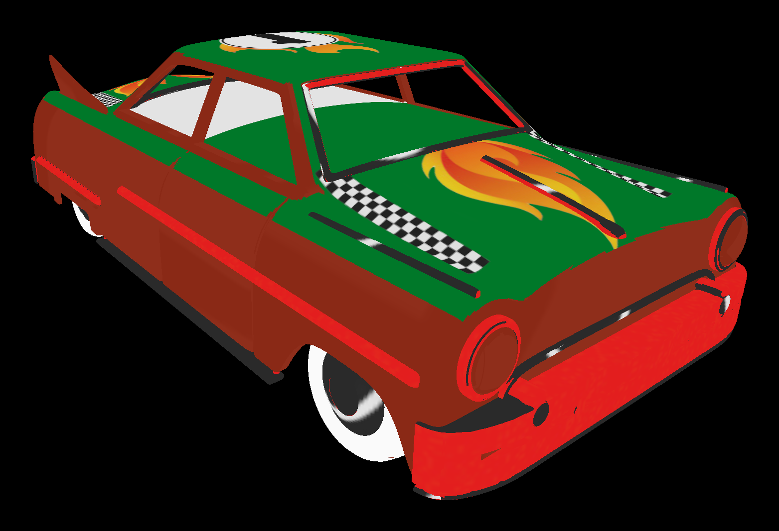
The companion lesson swaps one call for the textured variant, gltfModelWithTextureHere(path), which also binds the file's images as the sampler array uTextures the fragment shader declares: the array-of-samplers pattern above, filled from the file rather than by hand. The array gets exactly as many images as the shader declares, so the car's ten fill its six slots with the first six:
Render to texture
Everything so far drew into the window. RenderToTexture gives a module somewhere else to draw: an offscreen image that a later box can sample. It is the building block for post-processing, feedback, and anything that needs to read what it just drew.
The producing box creates the target, registers it on the renderer's render list, and attaches its module to the target rather than to the renderer:
prop<RenderToTexture>(target) = RenderToTexture {
    clearFirst = false
    useDepth = true
}

renderer.renderList += "target" to target

var module = moduleHere {
    // Match the module's pipeline (colour format, depth) to the target it draws into.
    +target
}
var m = Mesh()

module += "mainMesh" to m
target += "boo" to module

val camera = Camera()
m.p = camera.p
m.m = camera.m

// we can set this live and after the fact
target.parameters.clearFirst = true

var kc by keyCamera(camera = camera)
loop {
    m.set(3, 1) {
        val z = Math.random() * 0.0
        pos.add(-3, 1, -1 + z, 1.0, -20.3, z, 3, 3, z)
        tri.add(0, 1, 2)
    }
    true
}
Three lines carry the idea. renderer.renderList += "target" to target schedules the offscreen pass. target += "boo" to module puts the drawing inside that pass instead of on screen. And target.parameters.clearFirst = true shows that the target's parameters stay live: you can flip them from the editor while the loop is running, with no rebuild.
The consuming box is a child of the producer, and that is the whole binding mechanism:
prop<RenderToTexture>(bbc) = target

var module = moduleHere()
var mesh = Mesh()
module += "mainMesh" to mesh
renderer += "boo" to module

val camera = Camera()
camera.at = vec(0, 0, -1.2)
mesh.p = camera.p
mesh.m = camera.m

var kc by keyCamera(camera = camera)
mesh.set(4, 2) {
    val z = 0.0
    pos.add(-1, -1, z, 1.0, -1.0, z, 1, 1, z, -1.0, 1, z)
    tc.add(0, 0, 1, 0, 1, 1, 0, 1)
    tri.add(0, 1, 2)
    tri.add(0, 2, 3)
}
prop<RenderToTexture>(bbc) = target reads target (the parent's property, visible by name because this box is a child) and republishes it as bbc, because this box's fragment shader declares sampler2D bbc. Republication can rename freely: the resource is identified by the reflected name the consuming shader asks for, not by the name it was published under upstream, so a box can bind any upstream target to whatever its own shader happens to call it.
#version 450
layout(location = 0) out vec4 uFragColor;
layout(location = 1) in vec2 ftc;

layout(set=0, binding = 0) uniform sampler2D bbc;

void main()
{
    vec4 c = texture(bbc, ftc.yx);
    uFragColor = vec4(c.rgb, 1.0);
}
Compare that with the texturing fragment shader: it is the same shader. From the consumer's side there is no difference between sampling a file loaded from disk and sampling the output of another box. Two boxes and one renamed property are the smallest complete statement of how Field 4 composes.
threebox and spin_glass, from the agent transcripts, are runnable versions of the same producer/consumer shape.
Ping-pong render to texture
A target you can read and write in the same pass is a contradiction, so feedback needs two images with the roles swapped every frame. PingPongRenderToTexture does that bookkeeping:
import org.lwjgl.vulkan.VK10.*

prop<PingPongRenderToTexture>(target) = PingPongRenderToTexture {
    clearFirst = false
    useDepth = false
}

prop<HasImageView>(otherView) = target.otherImageView

renderer.renderList += "target" to target

var module = moduleHere {
    +target
}
var m = Mesh()

module += "mainMesh" to m
target += "boo" to module
target.otherImageView is the image that is not the current render destination, published as otherView so the fragment shader can sample last frame while writing this one:
layout(set=0, binding = 0) uniform sampler2D otherView;

void main()
{
    vec2 tc = gl_FragCoord.xy / 1024.0;
    vec2 px = vec2(1.0 / 1024.0);

    // Last frame, blurred hard and faded a little.
    vec3 c = vec3(0);
    float total = 0.0;
    for (int y = -1; y <= 1; y++)
        for (int x = -1; x <= 1; x++) {
            float w = (x == 0 && y == 0) ? 4.0 : ((x == 0 || y == 0) ? 2.0 : 1.0);
            c += w * texture(otherView, tc + 5.0 * px * vec2(x, y)).rgb;
            total += w;
        }
    c = c / total * 0.996;

    // A dot on a Lissajous path, its colour cycling, stamped in every frame.
    vec2 at = vec2(0.5) + 0.32 * vec2(cos(pc.time * 0.9), sin(pc.time * 1.3));
    vec3 ink = 0.5 + 0.5 * cos(pc.time + vec3(0, 2, 4));
    c = max(c, ink * smoothstep(0.025, 0.0, length(tc - at)));

    uFragColor = vec4(c, 1.0);
}
Each frame reads the last one blurred and slightly darker, then stamps the dot in at its new place, so the dot leaves a trail that spreads and fades rather than a line. pc.time advances a fixed 1/60 s per frame (m.time = { time += 1f / 60; time }), not with the clock, so a slow frame slows the animation instead of making the dot jump. The consuming box then displays target.thisImageView, the half that was just written:
prop<HasImageView>(bbc) = target.thisImageViewNote the property type here is HasImageView, not RenderToTexture. A ping-pong target is not one image, so the two halves are handed out individually, and HasImageView is the interface that any bindable image satisfies. module { +target } inside the module builder is what matches the module's pipeline state (format, sample count, attachment layout) to the target it draws into; without it the pipeline and the target disagree.
And the feedback running in the window: a dot moving through the target leaves a trail that blurs and fades, because each frame reads the last.
Replacing carried history at a playback cut
For a prepared cut, target.recordReplaceHistory(command, attachment) { image -> … }
records a transfer into every slot of one attachment's history ring. The callback records a
buffer-to-image or image-to-image copy into the supplied Vulkan image, in
TRANSFER_DST_OPTIMAL, covering mip 0 and every array layer. Its source must be separate from
the ring. Create the target with colorTransferDst = true, colorSampled = true and one mip
level, and call outside a render pass on the graphics recording thread.
Replacing all slots prevents an earlier frame from reappearing in feedback after the cut.
The other attachments, ring indices, bound attachment and cadence stay as they were. This
works on both PingPongRenderToTexture and FrameCadencedPingPongRenderToTexture.
renderer.whenCurrentGraphicsFrameComplete { … }, called while recording that graphics
frame, reports completion after its submission fence signals. Keep the callback short: complete
a future or hand work to an IO worker. The transfer method records commands without waiting;
prepare source resources before the cut. Neither method loads a snapshot from disk or captures
the rest of an application's simulation state.
A blur kernel across three boxes
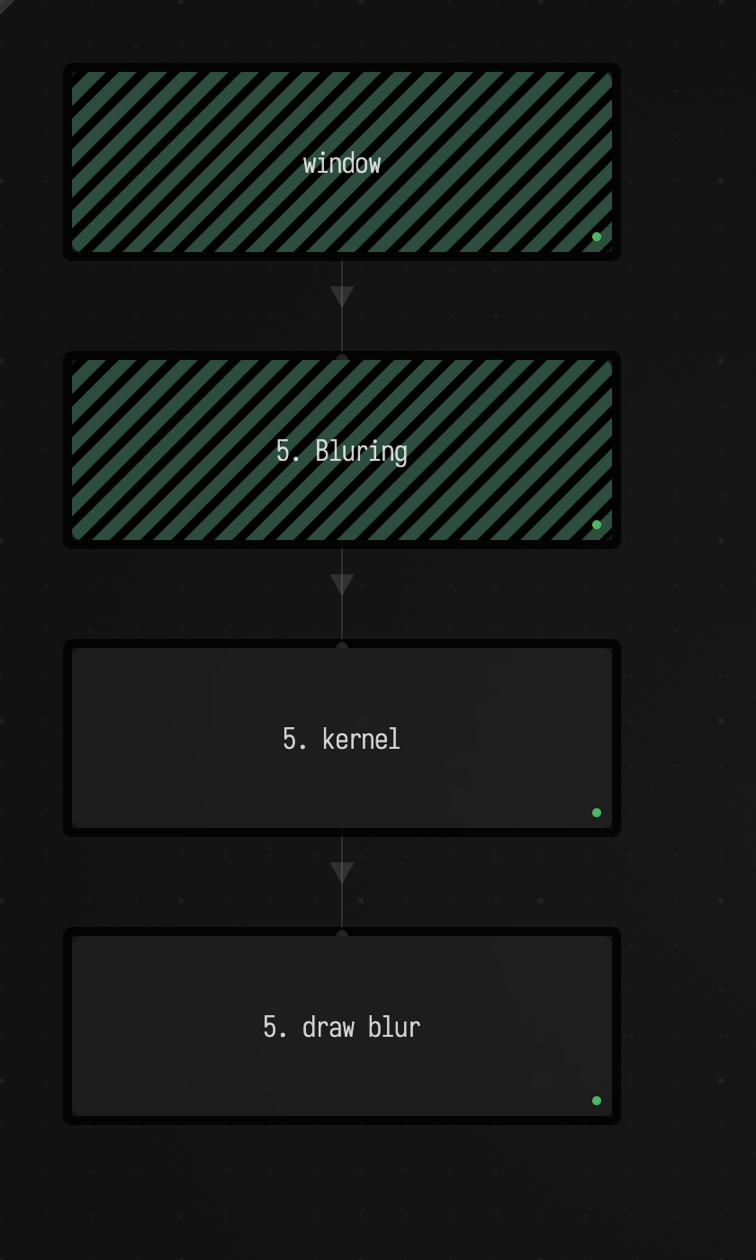
The blur chain is the longest topology in the corpus (window → 5. Bluring → 5. kernel → 5. draw blur), and it reads best as a whole, because each box does exactly one thing.
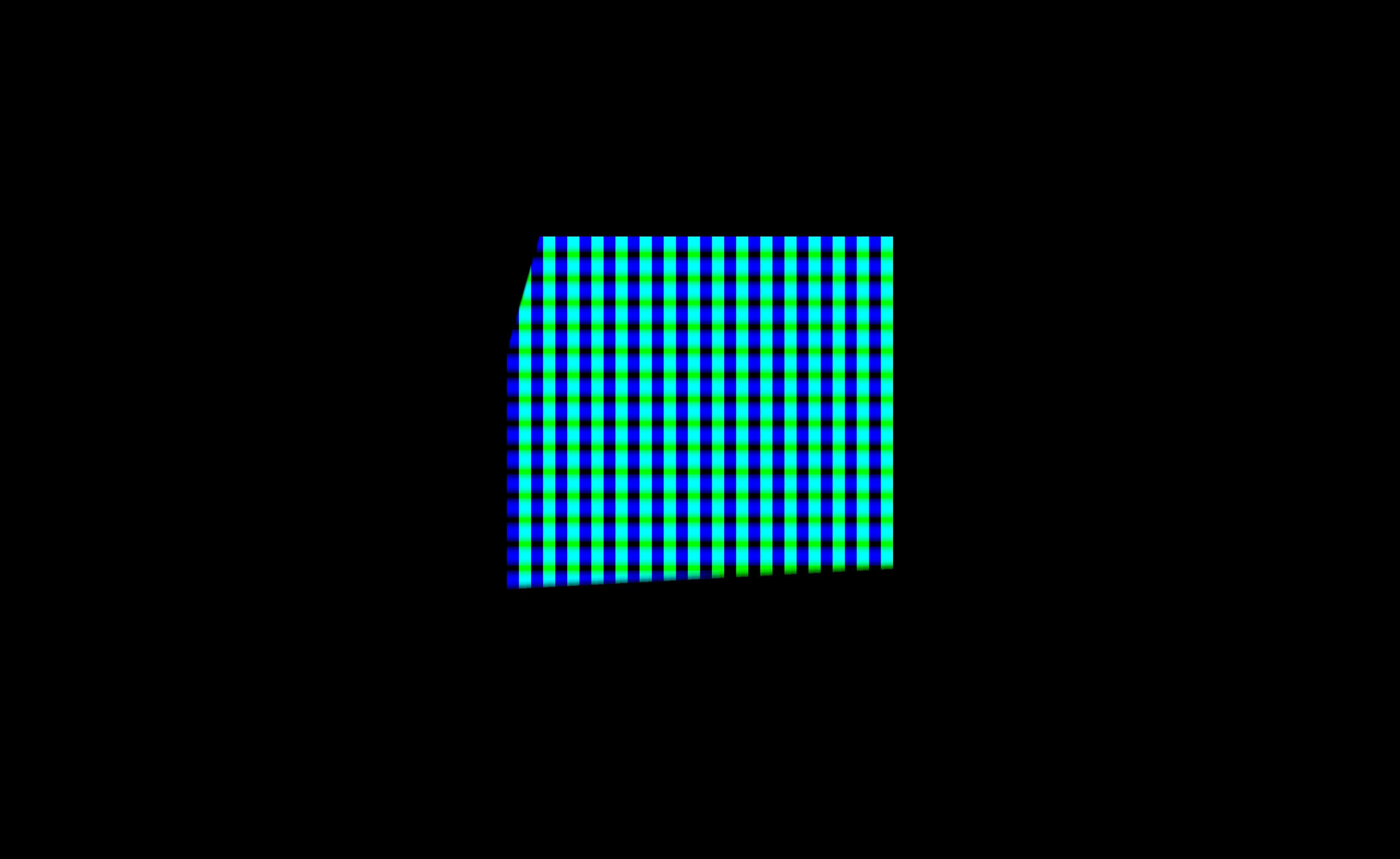
5. Bluring is a plain RenderToTexture producer like the one above, drawing a checkerboard so there is something with hard edges to blur:
void main()
{
    uFragColor = vec4(int(gl_FragCoord.x/32) % 2,int(gl_FragCoord.y/32) % 2,0,1);
}
5. kernel reads that target as b0, and renders into a second target of its own with two colour attachments and mip levels:
prop<RenderToTexture>(b0) = target

prop<RenderToTexture>(b1) = RenderToTexture {
    useDepth = false
    mipLevels = 10
    colorLayerCount = 2
    colorAttachments = 2
}

renderer.renderList += "b1" to b1

var module = moduleHere {
    primitiveType = triangle_strip
    depth = 0
    +b1
}

var m = Mesh()
module += "mainMesh" to m
b1 += "boo" to module

m.radius = { 10.0f }
m.sigma = { 10.0f }
m.resize(4)
m.resize(4) with no set block and primitiveType = triangle_strip is the fullscreen-quad idiom: four vertices, positions synthesized in the vertex shader from gl_VertexIndex, no vertex attributes at all. m.radius and m.sigma are reflected push-constant members, so the kernel's parameters are ordinary Kotlin lambdas you can edit live.
The interesting choice is in the vertex shader, which computes the Gaussian weights per vertex (four invocations instead of one per pixel) and passes them down as interpolants:
float gauss(float x, float sigma) {
    float s2 = sigma * sigma;
    return exp(-x * x / (2.0 * s2));
}

void main()
{
    float r1 = blur.radius * 0.275; // near
    float r2 = blur.radius * 0.65; // mid
    float r3 = blur.radius * 0.95; // far

    float w0 = gauss(0.0, blur.sigma);
    float w1 = gauss(r1, blur.sigma);
    float w2 = gauss(r2, blur.sigma);
    float w3 = gauss(r3, blur.sigma);
    float norm = w0 + 2.0 * (w1 + w2 + w3);

    radii = vec4(r1,r2,r3,norm);
    weights = vec4(w0,w1,w2,w3);

    vec2 p = positions[gl_VertexIndex];
    gl_Position = vec4(p, 0.0, 1.0);
    ftc = p * 0.5 + 0.5;

    gl_Layer = 1;
}
The weights are constant across the quad, so interpolating them is free and the four exp calls replace one per pixel. gl_Layer = 1 (with GL_ARB_shader_viewport_layer_array) picks which layer of the multi-layer target this pass writes.
The fragment shader is then a seven-tap symmetric blur that writes two attachments at once:
void main()
{
    vec2 texel = 1.0 / vec2(textureSize(b0, 0));
    vec2 dx1 = texel * vec2(radii.x, 0.0);
    vec2 dx2 = texel * vec2(radii.y, 0.0);
    vec2 dx3 = texel * vec2(radii.z, 0.0);

    vec4 c =
    weights.x * texture(b0, ftc)
    + weights.y * (texture(b0, ftc + dx1) + texture(b0, ftc - dx1))
    + weights.z * (texture(b0, ftc + dx2) + texture(b0, ftc - dx2))
    + weights.w * (texture(b0, ftc + dx3) + texture(b0, ftc - dx3));

    uFragColor = vec4(c.rgb / radii.w, 1.0);
    uFragColor1 = vec4(c.bgr / radii.w, 1.0);
}
Two layout(location = …) out declarations correspond to the colorAttachments = 2 on the Kotlin side. Finally 5. draw blur picks a specific layer out of the array to display:
prop<RenderToTexture>(bbc) = b1
val other = b1.imageViewArray[1]
prop<HasImageView>(back) = other
and samples it as a sampler2DArray, the type a layered target reflects as:
layout(set=0, binding = 0) uniform sampler2DArray bbc;
layout(set=0, binding = 1) uniform sampler2DArray back;

void main()
{
    vec4 c = texture(back, vec3(ftc.yx,1.0), 0.0);
    uFragColor = vec4(c.rgb, 1.0);
}
Here is the chain on the canvas:
and what the last box draws:
Shader includes
Shader properties are templated before they reach the compiler, and {% property "name" %} pulls in another property by name. 5. included shares its attribute and push-constant declarations with a sibling box:
#version 450

{% property "vertex_included" %}

layout (location = 0) out vec4 fcol;

void main()
{
    gl_Position = pc.p * pc.m * vec4(pos, 1);

    fcol = col;
}
where the included property is a fragment of GLSL with no main and no #version of its own:
layout (location = 0) in vec3 pos;
layout (location = 1) in vec4 col;
layout(push_constant) uniform matrices {
    mat4 p;
    mat4 m;
} pc;
Reflection happens after the include is expanded, so pos, col, p and m still produce the generated Kotlin writers: a shared header does not cost you the reflected API. The include resolves against a box that has to exist alongside the one including it, so this pair only compiles once both boxes are in the document.
5. lygia shows the same mechanism reaching a third-party shader library. registerLygiaIncludeRoot() in Kotlin registers Lygia's source tree as an include root, after which the shader uses ordinary #include:
#include "lygia/generative/gerstnerWave.glsl"
#include "lygia/generative/fbm.glsl"

void main()
{
    vec2 uv = ftc.xy * 1.0;
    vec3 f = gerstnerWave(uv, vec2(1.0, 1.2), 10.3, 0.3, 0.3);

    float n = fbm(uv*2 + f.yx * 0.75);
    float n2 = fbm(uv * 2.0 -
    f.yx * 0.5 +
    vec2(-f.y, f.x)*n*9);

    vec3 col = abs(f) * (0.6 + 0.8 * n) + vec3(n2 * 0.25, n * 0.2, n * 0.35);
    uFragColor = vec4(col, 1.0);
}
This example needs a Lygia checkout on disk, which is why it carries no figure.
Shader templating
Beyond includes, a shader property is a template with values supplied from Kotlin. shaderTemplate["col"] publishes a map of Resolvers, and the shader substitutes them with {{ … }}:
// we can define this first
shaderTemplate["col"] = mapOf("fixedColor" to Resolver { "vec4(1,0.75,0,1)" })

// Run the declarations above first; rerun the module fragment to compile its generated shader interface.
//%-
var module = moduleHere {
    primitiveType = triangle_strip
}

var m = Mesh()

module += m named "my mesh"
renderer += module

m.set(3, 3) {
    pos.add(0, 0, 0, 0.5, 0, 0, 0.5, 0.5, 0)
    tri.add(0, 1, 2)
}
#version 450
layout(location = 0) out vec4 uFragColor;

layout(location = 0) in vec4 fcol;
void main()
{
    uFragColor = vec4({{ col.fixedColor }});
}
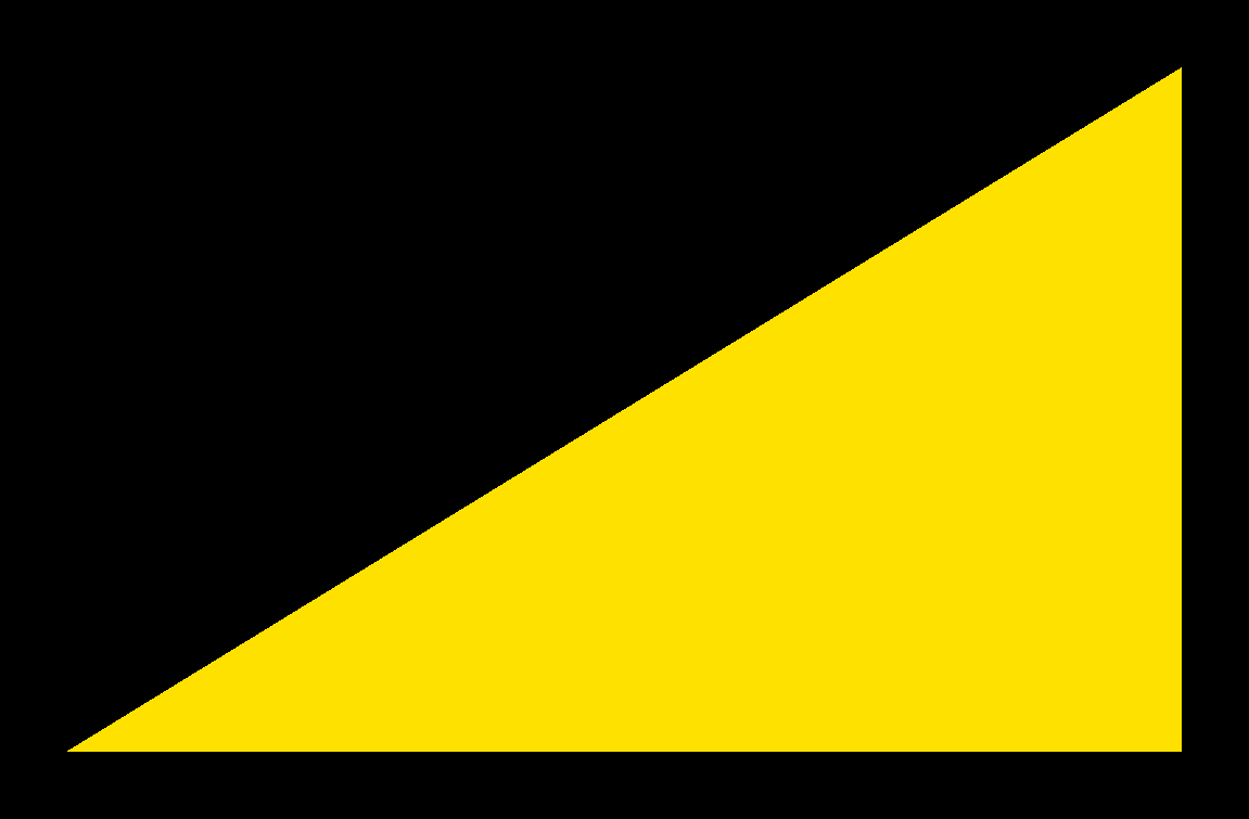
A Resolver is a lambda returning GLSL source, not a value: the string is spliced in before compilation, so {{ col.fixedColor }} becomes a compile-time constant rather than a uniform read. That is the trade: changing it recompiles the shader, and in exchange the optimiser sees a literal.
In the corpus this box also carries a //%- line, which is Field's execution break: everything above it runs once when the box is first evaluated, and the part below is what re-runs. Declaring the template before the break means the substitution is registered before moduleHere reads the shader.
Generated push-constant blocks
Templating gets more interesting when the substituted source is itself generated from a Kotlin type. PushConstants<T> reflects a Kotlin class into a GLSL push-constant declaration:
class MyPC(
    var a: Vec4,
    var b: Vec4,
    var c: Vec4,
) : PushConstants<MyPC>()

var pc = MyPC(vec(1, 0, 0, 1), vec(1, 2, 3, 4), vec(1, 2, 3, 4))

shaderTemplate["pc"] = mapOf("dec" to Resolver { pc.glsl() })

pc.a.x = 0.3f
pc.otherDeclarations = "layout(offset=${pc.nextFreeOffset(16)}) uint foo;"

// Run the declarations above first; rerun the module fragment to compile its generated shader interface.
//%-
var module = moduleHere {
    primitiveType = triangle_strip
}

var m = Mesh()

module += m named "my mesh"
renderer += module

m.push.bindAll { pc }
m.foo = { 10u }

m.set(3, 3) {
    pos.add(0, 0, 0, 0.5, 0, 0, 0.5, 0.5, 0)
    tri.add(0, 1, 2)
}
#version 450
layout(location = 0) out vec4 uFragColor;
layout(location = 0) in vec4 fcol;

{{ pc.dec }}
void main()
{
    loadRegs();

    uFragColor = vec4(a());
}
pc.glsl() emits the block declaration; {{ pc.dec }} splices it in; m.push.bindAll { pc } binds the whole Kotlin object to it in one call rather than member by member; and loadRegs() plus the accessor a() are part of the generated preamble, which is why the shader reads a() rather than pc.a. nextFreeOffset(16) computes where a hand-written extra member can sit without colliding with the generated layout, the escape hatch for the case the generator does not cover.
Debugging: printf from a shader
Vulkan can print from inside a shader. Enable the extension, guard the call so it does not fire for every invocation, and the message arrives through the validation layer:
var module = moduleHere { primitiveType = triangles }

var m = Mesh()
module += m named "someMesh"
renderer += module

var vertexData = defaultBuffer {
    perFrame = true
    size = 3.vec4s
}
    .buffer

m.vertexData = { vertexData }

vertexData.write {
    put(vec(0, 0, 0))
    put(vec(1, 0, 0))
    put(vec(0, 1, 0))
}

m.resize(3)
#version 450
#extension GL_EXT_buffer_reference : require
#extension GL_EXT_debug_printf : enable

// …

void main()
{
    vec3 pos = pc.vertexData.positions[gl_VertexIndex].xyz;
    gl_Position = vec4(pos, 1);

    localColor = vec4(wrap(gl_VertexIndex,3),wrap(gl_VertexIndex,5),wrap(gl_VertexIndex,11),1.0);

    if (gl_VertexIndex == 0) {
        debugPrintfEXT("VS: index=%d, pos=(%f,%f)",gl_VertexIndex, pos.x, pos.y);
    }
}
Two things are required. #extension GL_EXT_debug_printf : enable has to be there, and printing needs the validation layer (Options.validate, on by default, or Options.shaderDebugPrintf); a shader that calls debugPrintfEXT with both off gets a warning in the log, since it would print nothing. And the guard matters: debugPrintfEXT with no condition in a shader running over a million invocations will flood the log and stall the frame. The guard here (gl_VertexIndex == 0) prints once per draw, for the first vertex.
Debugging: texture probes
The other debugging tool goes the other way: instead of printing text, it samples a value out of a running shader and draws it. fieldProbeHere() creates the probe and {% property "fieldProbe" %} brings the shader side in:
prop<LoadedTexture>(bbc) = LoadedTexture("public/docs/assets/afield_four_graphics/docs-checker-texture.png")
bbc.transferNow()

var module = moduleHere {}
var m = Mesh()

val probe = fieldProbeHere().display("probe")

module += "mainMesh" to m
renderer += "boo" to module

val camera = Camera()
camera.at = vec(0.5, 0.5, -0.8)
camera.target = vec(0.5, 0.5, 0)
m.p = camera.p
m.m = camera.m

var kc by keyCamera(camera = camera)
val n = 100
m.set(4 * n, 2 * n) {
    n {
        val z = it + 0.0

        pos.add(0, 0, 0 + z, 1.0, 0.1, z, 1, 1, z, 0, 1, z)
        tc.add(0, 0, 1, 0, 1, 1, 0, 1)

        val b = it * 4
        tri.add(b + 0, b + 1, b + 2)
        tri.add(b + 0, b + 2, b + 3)
    }
}
#version 450

{% property "fieldProbe" %}

// …

void main()
{
    gl_Position = pc.p * pc.m * vec4(pos, 1);

    fieldProbe(gl_Position.xyz/gl_Position.w);

    ftc = tc;
}
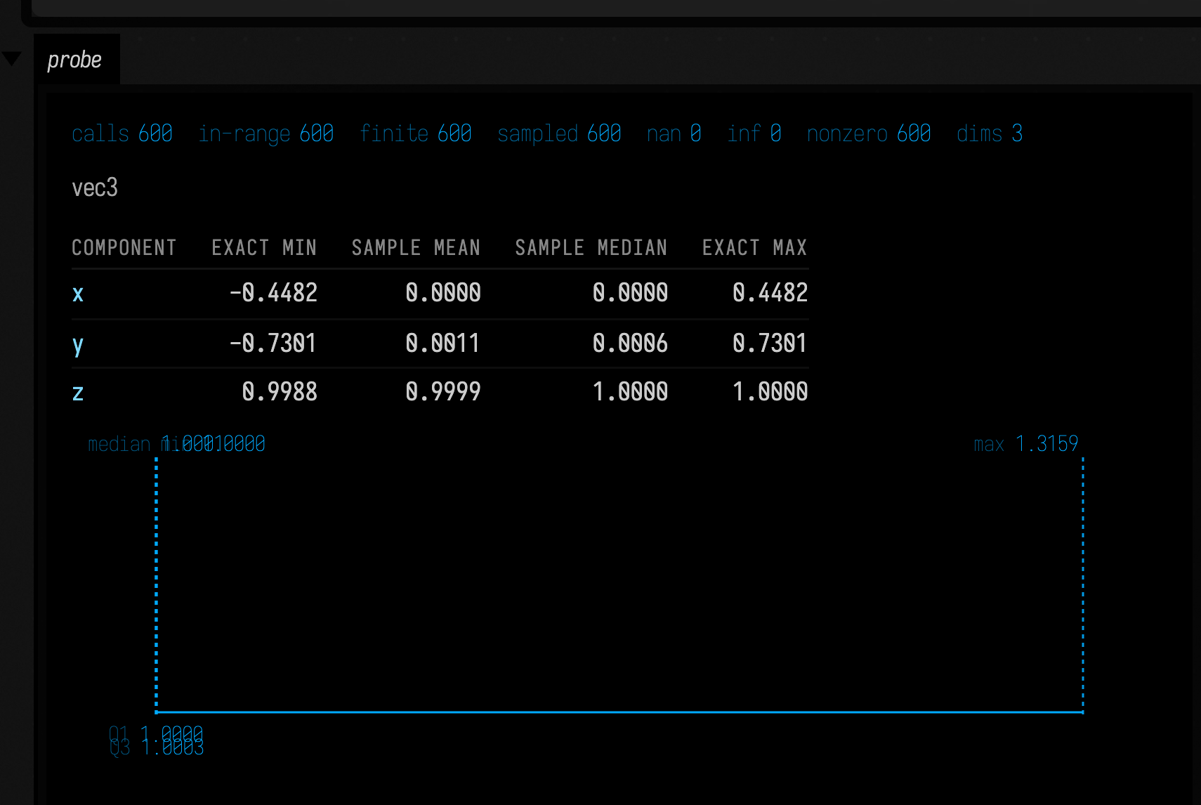
fieldProbe(…) writes the sampled value into a buffer the probe owns, and .display("probe") puts the readback in the box's output area. Probing the post-projection position, as here, is how you check a transform is doing what you think without reasoning backwards from the picture. n = 100 stacked quads make it worth probing: 400 vertices where a wrong p or m is otherwise just a blank window. See Field probes for the readback side.
A second probe lesson (6b. debugging / mapping - Texture probe example) goes further and warps the sampled distribution before display (AdaptiveQuantileWarp and QuantileWarpConfig). Reach for that when the interesting variation is buried in a narrow part of the range and a linear readout flattens it.
In the Vulkan window the 100 quads stack along z, so from the camera they land on top of one another and look like one. Everything this example is for is in the box's output area.
Streaming a target over the network
FieldRTTStreamer turns a render target into an encoded video stream, which is how a Field sketch drives a display it is not attached to. A render can also be streamed over WebRTC to other Field instances and to browser ShaderTrinkets (WebRTC Streams), or shown in Field's own desktop app (graphics in output areas). The largest consumer of FieldRTTStreamer is the Vision Pro front end; see Apple Vision Pro, which covers the stereo side-by-side layout, the media wire's pose tail, and tagPosesFrom for stamping a frame with the head pose it was rendered from:
import afield.media.stream.FieldRTTStreamer
import org.lwjgl.vulkan.VK10.*

// Streamer allocates + imports the surface and hands back the RTT to render into.

prop<FieldRTTStreamer>(streamer)
once.streamer {
    FieldRTTStreamer(renderer, dest = "127.0.0.1:9001", width = 1280, height = 720, fps = 15)
}

prop<RenderToTexture>(target) = streamer.start().first()

renderer.renderList += "target" to target

var module = moduleHere { +target }
var m = Mesh()
module += "mainMesh" to m
target += "boo" to module
The shape is exactly the RenderToTexture producer from earlier (renderList +=, target +=, +target) with the target supplied by the streamer instead of constructed directly. once.streamer { … } is the live-coding guard: re-running the box re-runs everything except the block that allocated the stream, so you can edit the drawing without tearing down the connection. prop<RenderToTexture>(target) = … publishes the target as a typed property, so child boxes inherit it as target the same way the particle draw box inherits outputPositions.
The picture this produces arrives at a receiver on 127.0.0.1:9001 rather than in a window.
A GPU radix sort
Not every compute job is a shader you write. GpuRadixSort is a prepackaged one, and this example is about how it schedules work rather than about the sort itself:
val sorter = GpuRadixSort()

var sourceBuffer = buffer {
    size = 200.ints
    storage()
    addressable()
    hosted()
    dest()
}
    .buffer

sourceBuffer.write {
    200 {
        putInt(2000 - it)
    }
}

renderer.renderList.others["sort"] = Target { command, index ->
    sorter.sort(command, sourceBuffer, 200)
}

sourceBuffer.read_ints {
    _print(this.get(0))
}
Two things to take from it. The buffer { … } builder spells out usage explicitly: storage(), addressable() (needed for buffer references), hosted() (CPU-visible), dest() (a transfer destination). Those flags are what decide whether a given access is legal later. And renderList.others["sort"] = Target { command, index -> … } is the general escape hatch: a slot on the frame where you get the command buffer and can record whatever Vulkan work you like. sorter.sort(command, …) records into that buffer rather than executing immediately.
This example reads back through hosted() memory. For a GPU→CPU read that happens every frame, use host-cached memory instead; see the readback notes in Field probes.
This box sorts and prints, and draws nothing.
Slang
The same box model accepts Slang instead of GLSL through the vertex_fragment property, which holds both stages in one file. The Kotlin side does not change at all: modules, meshes, buffers and reflected accessors work the same way, because reflection reads the compiled shader interface rather than the source language.
var module = moduleHere { primitiveType = triangles }

var m = Mesh()
module += m named "someMesh"
renderer += module

var vertexData = defaultBuffer {
    perFrame = true
    size = 3.vec4s
}
    .buffer

m.vertexData = { vertexData }

var t = 0.0
fun polar(t: Double, r: Double) = vec(Math.sin(t), Math.cos(t)) * r.f

loop {
    t += 0.01
    var num = 0

    var numVertToWrite = (Math.sin(t * 0.1) * 20 + 30).i

    vertexData.write {
        for (x in 0 until numVertToWrite) {
            val offset = vec(x * 0.02, 0, 0)
            put(vec(polar(t, 0.5), 0) + offset)
            put(vec(polar(t + 0.4, 0.4), 0) + offset)
            put(vec(polar(t + 0.9, 0.3), 0) + offset)

            num += 3
        }
    }

    m.resize(num)
    true
}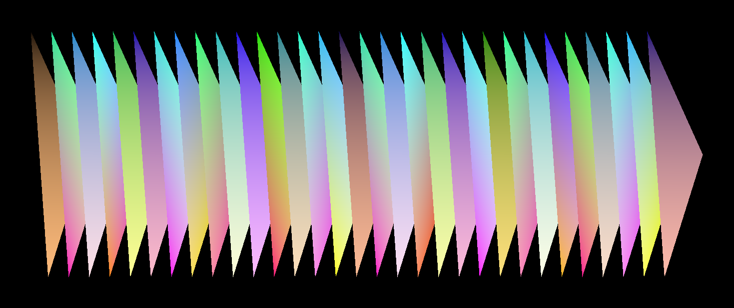
The corpus box for this lesson (7. slang — hello triangle) is also the best-commented file in the collection, and is written as a tutorial. Open it directly: it makes two points in passing that generalise beyond Slang. First, buffer sizes are a guess that Field will correct: size = 3.vec4s is set too small there, and the buffer resizes dynamically rather than failing. Second, perFrame = true allocates one buffer per frame in flight, so a write never has to wait on the GPU to finish reading.
A second Slang lesson (7b. slang — Texture) is the same step again with a texture bound, and it makes the language-independence claim concrete: the Kotlin is the texturing code from earlier, unchanged, prop<LoadedTexture> and all, because the resource is matched by reflected name and the name survives the change of shader language.
Slang requires slangc to be available. Field checks an explicit AFIELD_SLANGC or -Dafield.slangc override, then PATH, then the optional compiler prepared by ./gradlew buildLearnedShaders. That task uses a pinned shared cache; live compilation itself does not download anything. See the optional toolchain.
Diffusion-limited aggregation
The last lesson is the shortest, because the work is packaged:
var dla = ShaderDlaSystem() {
    width = 1024
    height = 1024
    particleCount = 300_000
}

// this installs editable shaders
dla.installInto()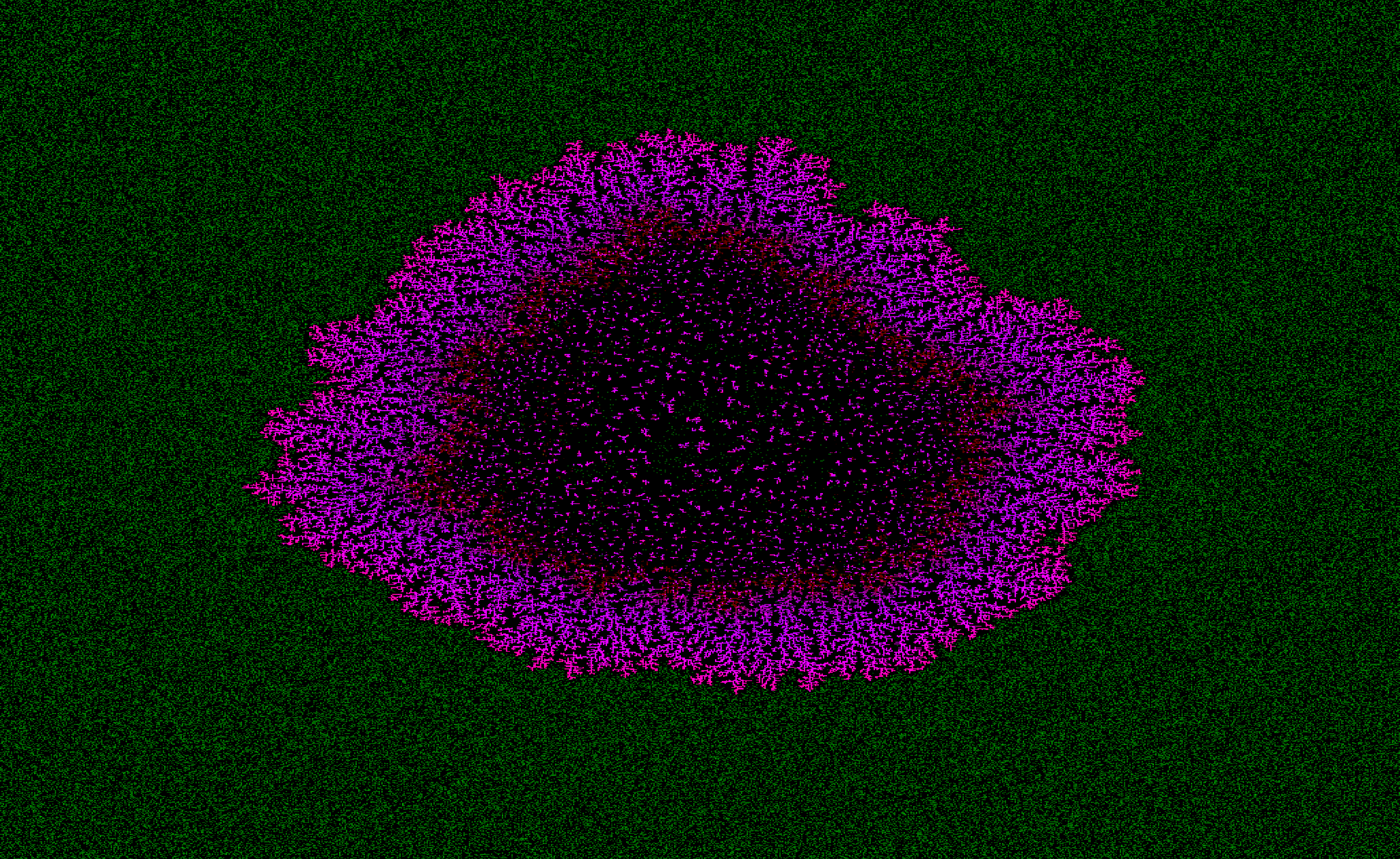
installInto() writes the system's shaders into this box's shader properties, so a packaged effect arrives as source you can edit rather than as a closed component. The vertex shader it installs is a million-particle random walk that reads the accumulated image as a texture, steps each walker, sticks it when it touches something solid, and writes the particle state back through a buffer reference: simulation and drawing in a single vertex shader, with no compute pass at all:
void main() {
    ivec2 dims = textureSize(sourceTex, 0);
    vec2 maxPos = vec2(max(dims.x - 1, 0), max(dims.y - 1, 0));

    Particle particle = push.particleBuffer.particles[gl_VertexIndex];
    uint rng = particle.rngState ^ (uint(gl_VertexIndex) * 2246822519u + 3266489917u);
    vec2 positionPx = clamp(particle.positionPx, vec2(0.0), maxPos);
    uint mode = particle.mode;
    bool becameSolid = false;

    if (mode != 0u) {
        positionPx = randomPosition(rng, dims);
        mode = 0u;
    }
    else {
        ivec2 center = clamp(ivec2(round(positionPx)), ivec2(0), dims - 1);
        int probe = max(int(round(push.sampleStepPx)), 1);
        bool solidNeighbor =
        isSolidAt(center + ivec2(probe, 0), dims, push.solidThreshold) ||
        isSolidAt(center + ivec2(-probe, 0), dims, push.solidThreshold) ||
        isSolidAt(center + ivec2(0, probe), dims, push.solidThreshold) ||
        isSolidAt(center + ivec2(0, -probe), dims, push.solidThreshold);

        if (solidNeighbor) {
            mode = 1u;
            becameSolid = true;
        }
        else {
            positionPx = clamp(positionPx + randomWalkStep(rng, push.walkStepPx), vec2(0.0), maxPos);
        }
    }

    push.particleBuffer.particles[gl_VertexIndex].positionPx = positionPx;
    // …
}push.walkStepPx, push.solidThreshold, push.stuckRed and the rest are reflected push-constant members, so every constant in the simulation is a Kotlin lambda away from being animated. The reflected-interface contract this page opened with still holds at a million particles: the shader is the thing you edit.
Whether the result branches depends on how densely the walkers cover the texture, and the useful range is narrow. The settings above, 300 000 walkers on 1024×1024 (about 0.3 per pixel), grow visible branches within 1500 frames and a cluster about 200 pixels across by 6000. A million walkers over a 4112×2524 window are too sparse: after 3000 frames the cluster is about a dozen pixels across. A million over 900×560, about two per pixel, are too dense to branch: every point of the cluster's edge has a walker beside it, so it grows as a solid diamond rather than a dendrite. At the density above solidDecayPerFrame makes little visible difference.
Traffic: the Biham–Middleton–Levine model
In the Biham–Middleton–Levine model every cell of a torus is empty or holds one car. Red cars only move right, blue cars only move down, and they take turns: on even steps every red car with an empty cell ahead moves into it, on odd steps the blue cars do the same. The only parameter is how many cars there are. Run this in a box beneath the renderer box:
var bml = ShaderBmlSystem() {
    width = 512
    height = 512
    density = 0.32f
}
bml.installInto()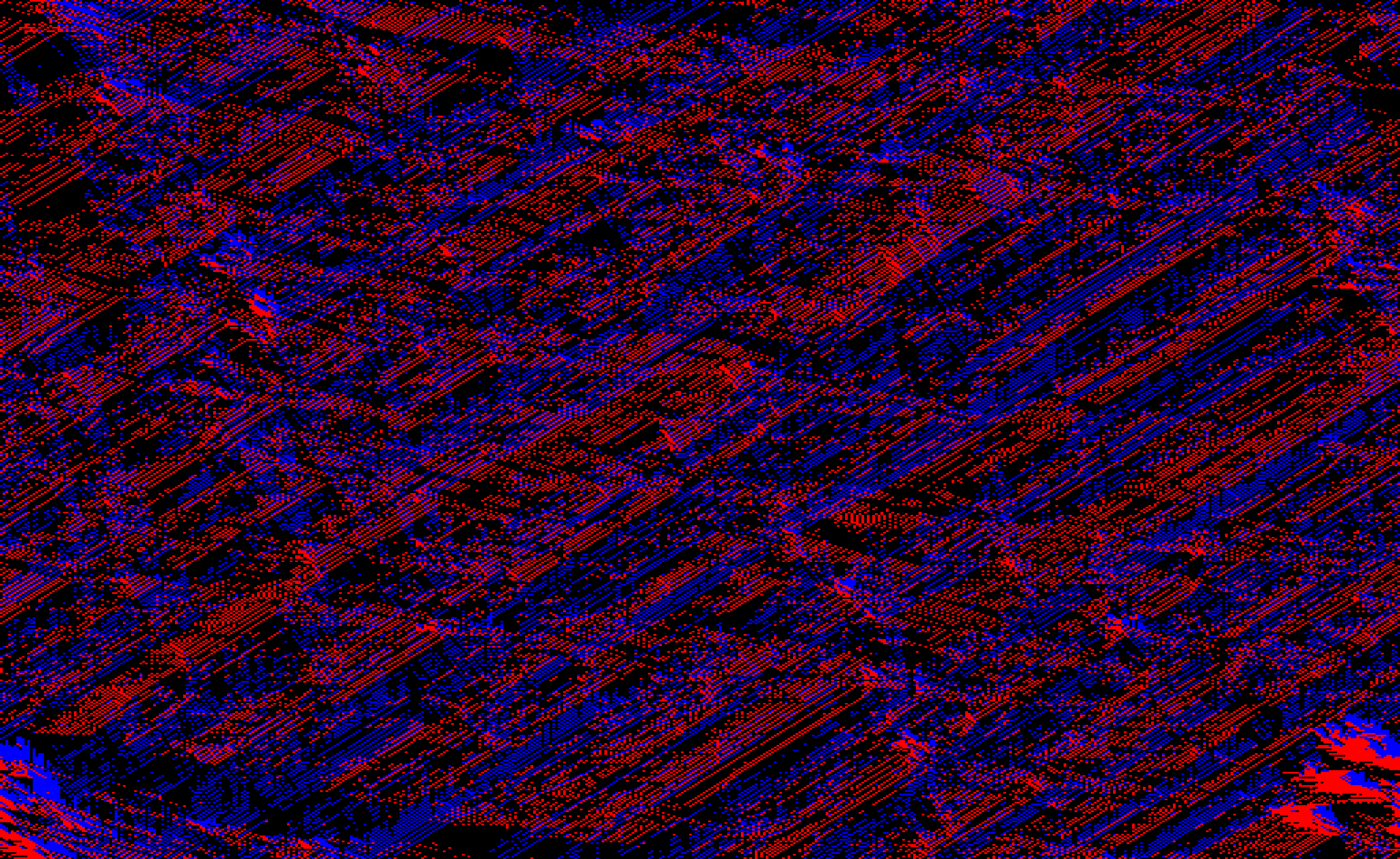
The grid appears in the renderer's window. This box, and the probed one below, are the 9. bml traffic and 9b. bml probe lessons of canonical_graphics. The cars start as noise and organise into diagonal bands within a few hundred steps. At 0.32 the bands then slowly lose: the fraction of cars moving falls from 0.92 to 0.44 over 2000 steps, because that density is close to the transition. At 0.20 the bands win and the moving fraction climbs to 0.998; at 0.45 a jam spanning the whole grid forms, and by step 1750 nothing moves. Change density and re-run, or call bml.reset() to scatter a new grid with the current settings. bml.settings.running = false pauses it.
The state is the texture, red at 1 for a red car and blue at 1 for a blue one, and each frame is one half-step: a full-screen pass that reads the previous frame and writes this one. Every cell decides from three texels. It empties if it holds a car of the moving colour and the cell ahead is empty, fills if it is empty and the cell behind holds one, and otherwise stays as it was. Because every cell gathers rather than any car pushing, no two cars can claim the same cell and the car count is conserved exactly. That rule is what the box's fragment tab holds, and editing it re-runs the model:
int mover = push.mode == 0 ? 1 : 2;
ivec2 ahead = push.mode == 0 ? ivec2(1, 0) : ivec2(0, 1);

int next = here;
if (here == mover && cellAt(p + ahead, dims) == 0) {
    next = 0;
    // a car moves out of this cell this half-step ...
}
else if (here == 0 && cellAt(p - ahead, dims) == mover) {
    next = mover;
}

outColor = colourOf(next);
Probing the cars that move
The window shows the pattern but not how much of the traffic is moving. A field probe can tell you. Set probe to a GLSL expression and the system calls fieldProbe(...) with it at the commented line above, which runs exactly once for each car that moves. Here it records x + y of the cell the car is leaving:
var bml = ShaderBmlSystem() {
    width = 512
    height = 512
    density = 0.32f
    probe = "float(p.x + p.y)"
}
bml.installInto()

fieldProbeHere(samples = 4096).display("probe")
displayOpen("probe")
The card on the box's probe channel shows two things. Its calls count is exactly how many cars moved this half-step. Divide it by the number of cars of one colour (density × width × height / 2 at the default even split) and you have the model's mean velocity, the usual measure of the jamming transition: near 1 in free flow, 0 in a jam. The histogram is the distribution of x + y over the moving cars. Cars scattered uniformly would give a triangle peaking in the middle of the range, and the diagonal bands show up as departures from that triangle while they form.
probe writes the instrumented rule into the fragment tab, replacing what was there, so to probe something else you can edit the call in place. The tab then reads:
#version 450

layout(set = 0, binding = 0) uniform sampler2D sourceTex;

layout(push_constant) uniform Push {
    int mode;
    float density;
    float eastboundFraction;
    int seed;
} push;

{% property "fieldProbe" %}

layout(location = 0) out vec4 outColor;

const vec4 EMPTY = vec4(0.0, 0.0, 0.0, 1.0);
const vec4 EAST = vec4(1.0, 0.0, 0.0, 1.0);
const vec4 SOUTH = vec4(0.0, 0.0, 1.0, 1.0);

uint hash(uint x) {
    x ^= x >> 16u;
    x *= 0x7feb352du;
    x ^= x >> 15u;
    x *= 0x846ca68bu;
    x ^= x >> 16u;
    return x;
}

float random01(uvec2 p, uint salt) {
    return float(hash(p.x ^ hash(p.y ^ hash(uint(push.seed) ^ salt)))) / 4294967295.0;
}

// 0 empty, 1 eastbound, 2 southbound
int cellAt(ivec2 p, ivec2 dims) {
    vec4 c = texelFetch(sourceTex, (p + dims) % dims, 0);
    if (c.r > 0.5) return 1;
    if (c.b > 0.5) return 2;
    return 0;
}

vec4 colourOf(int cell) {
    return cell == 1 ? EAST : (cell == 2 ? SOUTH : EMPTY);
}

void main() {
    ivec2 dims = textureSize(sourceTex, 0);
    ivec2 p = ivec2(gl_FragCoord.xy);

    if (push.mode == 3) {
        uvec2 u = uvec2(p);
        if (random01(u, 1u) < push.density) {
            outColor = random01(u, 2u) < push.eastboundFraction ? EAST : SOUTH;
        }
        else {
            outColor = EMPTY;
        }
        return;
    }

    int here = cellAt(p, dims);
    if (push.mode == 2) {
        outColor = colourOf(here);
        return;
    }

    // even half-steps move eastbound cars +x, odd ones move southbound cars +y
    int mover = push.mode == 0 ? 1 : 2;
    ivec2 ahead = push.mode == 0 ? ivec2(1, 0) : ivec2(0, 1);

    int next = here;
    if (here == mover && cellAt(p + ahead, dims) == 0) {
        next = 0;
        fieldProbe(float(p.x + p.y));
        // a car moves out of this cell this half-step: one invocation per moving car,
        // which is where to tap it (fieldProbe, fieldStats) without counting it twice
    }
    else if (here == 0 && cellAt(p - ahead, dims) == mover) {
        next = mover;
    }

    outColor = colourOf(next);
}
A fluid: lattice Boltzmann
ShaderLatticeBoltzmannSystem is a two-dimensional fluid. Every texel is a lattice site holding nine numbers, how much fluid there is moving in each of nine directions: still, the four neighbours, the four diagonals. A step moves each of those one site along its direction, then relaxes each site toward the equilibrium for its own density and velocity, and a population that runs into a solid site bounces back where it came from. Density and velocity are never stored; they are sums over the nine. This box builds one as a wind tunnel, wind blowing left to right across a lattice that wraps:
/*
A lattice Boltzmann fluid in a wind tunnel: a wind blows left to right and the
lattice wraps, so what leaves on the right comes back on the left.
On its own it is uniform wind and shows nothing; the box beneath this one puts
something in its way.
*/
prop<ShaderLatticeBoltzmannSystem>(lbm) = ShaderLatticeBoltzmannSystem() {
    width = 800
    height = 480
    baseVelocity = Vector2f(0.08f, 0f)
    // a thin fluid (viscosity about 0.014) so the wake sheds vortices
    relaxation = 1.85f
    // nothing pulls the fluid back toward the wind, so the wake travels;
    // the inlet that 10b draws at the left edge keeps the wind blowing
    driveBlend = 0f
    stepsPerFrame = 8
    dyeDecayPerFrame = 0.001f
    // vorticity: orange turns one way, blue the other. Try COMPOSITE, DYE or SPEED
    previewMode = FluidVisualizationMode.CURL
}

// this installs the editable collision-and-streaming rule in this box's fragment tab
lbm.installInto()
A wind through an empty tunnel is uniform and shows nothing, so a second box beneath this one puts something in its way. It draws into the fluid's control texture, where red is solid, green and blue a push, and alpha a dye source that also holds the wind steady. controlsParameters gives the module additive blending, and the controls are carried from frame to frame, so what the shader writes is a drawing that stays until clearControls() erases it:
/*
Draws into the fluid's control texture: a solid disc, walls top and bottom, and
stripes of dye released at the left edge. The controls persist from frame to
frame, so clear them first or a re-run leaves the old drawing behind.
*/
lbm.clearControls()

var module = moduleHere(lbm.controlsParameters("cylinder"))
lbm.addControls("cylinder", module)

val quad = fullscreenTriangle(module)
module += "quad" to quad

quad.center = { vec(160f, 236f) }
quad.radius = { 24f }
quad.height = { 480f }
void main() {
vec2 p = gl_FragCoord.xy;
outColor = vec4(0.0);
if (distance(p, push.center) < push.radius) outColor.r = 1.0;
if (p.y < 3.0 || p.y > push.height - 3.0) outColor.r = 1.0;
if (p.x < 4.0 && mod(floor(p.y / 12.0), 2.0) == 0.0) outColor.a = 1.0;
}These are the 10. lattice boltzmann and 10b. lbm cylinder lessons of canonical_graphics, and the lattice_boltzmann_cylinder starting point builds both with their renderer. The flow divides round the cylinder, and within a minute or so the two layers of shear behind it start to roll up alternately, one turning each way, and leave a von Kármán vortex street:
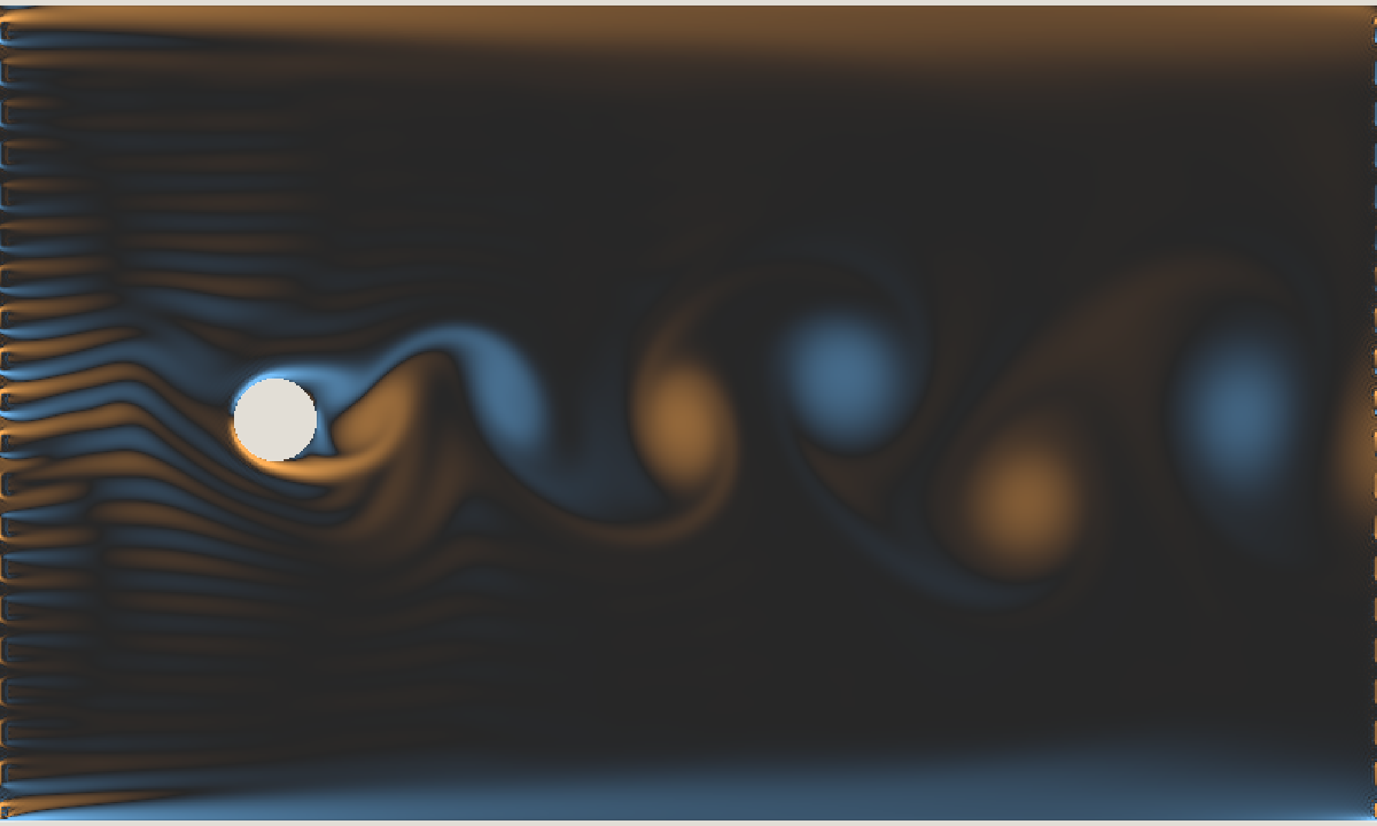
What decides it is the Reynolds number, speed times cylinder width over viscosity. The viscosity is (1/relaxation − 0.5) / 3, so relaxation = 1.85f gives about 0.014 and, with a wind of 0.08 sites per step past a 48-site cylinder, a Reynolds number near 280. Two settings in this box are there to let the street form. driveBlend = 0f turns off the pull back toward the wind that every site otherwise feels, which would damp a growing wake faster than it grows; the inlet stripes keep the wind blowing instead. And initialNoise, on by default, starts the fluid with a velocity too small to see, because a symmetric setup computed exactly stays symmetric and the wake would never start to swing.
stepsPerFrame = 8 runs eight lattice steps a frame. The method is only accurate while the fluid moves well under a site per step, so at one step a frame a gust takes thousands of frames to cross the window. previewMode chooses what you see: CURL is vorticity, DYE the dye alone, SPEED and VELOCITY the flow, COMPOSITE the dye lit by the flow. It is read every frame, so assigning lbm.settings.previewMode from another box changes the view without restarting anything, and so does every other setting except the sizes.
The box's fragment tab holds one step of the method, all nine populations written to three attachments of one ping-pong target in a single pass, and editing it re-runs the fluid.
A forest fire
ShaderForestFireSystem spreads fire through a forest. Each texel is a tree or bare ground, decided once from a hash of its position, and each tree is ready to burn, burning, or recovering. A ready tree catches from a burning neighbour, by chance: each burning neighbour gets one try per frame with probability spreadProbability, half by default. A tree burns for a few frames, then cannot burn again until it has recovered. Because trees recover, the fire never runs out of fuel, and a front can be followed by another one through the same trees. There are four kinds of fire, one per colour channel, and they compete: a tree that catches one kind is not available to the others until it has recovered. This box builds a forest the shape of the window:
/*
A forest fire: a fixed scatter of trees, and four kinds of fire (red, green, blue,
magenta) that compete for them. Burnt trees recover, so a fire front can be
followed by another. Nothing burns until something is lit; the box beneath this
one lights it.
The forest is 768 trees high and as wide as the window's shape needs, so it fills
the window without being stretched.
*/
val treesHigh = 768
prop<ShaderForestFireSystem>(fire) = ShaderForestFireSystem() {
    height = treesHigh
    width = treesHigh * window.width / window.height
    treeDensity = 0.6f
}

// this installs the editable spreading rule in this box's fragment tab
fire.installInto()
Nothing burns until something is lit. The box beneath it draws into the fire's ignition texture, one kind of fire per channel; fireInputParameters makes the drawing additive, so writing 1 into a channel lights that kind there. This one lights two points, red and green, and keeps them lit:
/*
Draws into the fire's ignition texture: two points that burn for ever, one red
and one green. Each relights its neighbourhood as soon as the trees recover, so
each sends out a train of rings, and where the trains meet one kind takes over.
*/
fire.clearFireInput()
fire.clearState()

var module = moduleHere(fire.fireInputParameters("starter"))
fire.addFireInput("starter", module)

val quad = fullscreenTriangle(module)
module += "quad" to quad

// positions are in trees, so place them as fractions of the forest's size
val w = fire.settings.width.toFloat()
val h = fire.settings.height.toFloat()
quad.red = { vec(w * 0.33f, h * 0.5f) }
quad.green = { vec(w * 0.68f, h * 0.5f) }
quad.radius = { 4f }
void main() {
vec2 p = gl_FragCoord.xy;
outColor = vec4(0.0);
if (distance(p, push.red) < push.radius) outColor.r = 1.0;
if (distance(p, push.green) < push.radius) outColor.g = 1.0;
}These are the 11. forest fire and 11b. fire starter lessons of canonical_graphics, and the forest_fire starting point builds both with a square window of their own. A point that never goes out relights the trees round it as soon as they recover, so each sends out a train of rings, one ring per recovery time. Red recovers faster than green by default, so its rings come more often. The two trains meet, and in the trees between the sources they interleave, each kind taking the trees the other has just left:
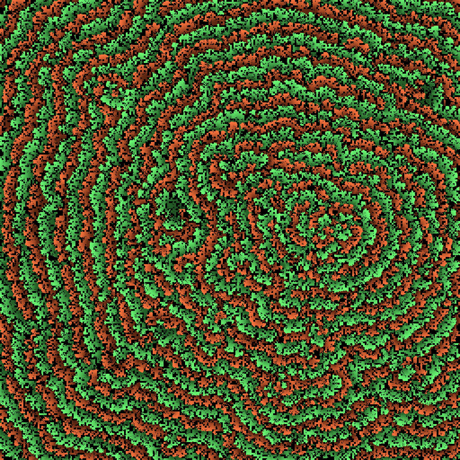
spreadProbability is what makes the rings round. At 1 every burning tree lights all eight of its neighbours at once, the fire moves one texel a frame along the diagonals as fast as along the axes, and the rings come out square. At one half each front advances by chance, slower on average, and roughens into a ragged circle. treeDensity is the other setting to try: it is the fraction of texels that hold a tree, and the default of 0.72 makes a denser, more uniform forest than the 0.6 here.
The box's fragment tab holds the spreading rule, and editing it re-runs the fire.
Stopping the renderer
Stopping the box that owns renderer also stops every running box connected beneath it, then
frees the GPU device. The same happens when you close the Field window. Field waits up to two
seconds for those boxes to finish; a loop {} stops within a frame. So a child box that writes
buffers every frame does not outlive the memory it writes into.
To start them again, select the renderer box and run Relaunch the N box(es) stopping this
renderer stopped from the command palette. It launches the renderer box first if its renderer
is gone, then the boxes it stopped, parents before children.
Anything that is not a box job, such as a raw thread {} or a renderer stashed in a global, is
not stopped. If it writes a buffer after the device is gone, it gets an IllegalStateException
that says so. A queue submission after the renderer has gone, or a descriptor that still names a
freed buffer, is refused the same way. Stop that work yourself, from a box you can stop.
Agents: teardown order
The shutdown order is written up in dev_docs/renderer_teardown_order.md.
Where these examples come from
Every example on this page is a box in a real Field document, canonical_graphics, which is what
the viewer at the top of this page is showing. To read the code rather than the prose, click a box
there for its Kotlin, its shaders and the picture its window drew, or
open the document full-page. To run and
edit the lessons, open Welcome → Starting points → canonical_graphics in Field, which makes you
an editable copy; launch its window box first, then a lesson.
Agents: the lesson index
Before writing Field 4 graphics code, adapt a lesson from
LESSONS.md. It lists every lesson with its Kotlin and
shader files, records the parent chain each one needs in order to run, and carries a reverse
index from Field API name (RenderToTexture, LoadedTexture, computeModuleHere,
GpuRadixSort, …) to the lessons that use it.
Each image is the lesson's own output, captured from a live Vulkan window. Sections without an image say why under the code: the lesson needs two boxes wired together, needs a file or tool the repository does not ship, or produces something other than a picture. For the two-box shape, the threebox and spin_glass agent transcripts are runnable versions.
Fabricate Renderer
For experimental area lights, Vulkan ray-query shadows and optional RTXDI resampling, see Direct lighting. Other pages that build on the pieces here:
- Ray Tracing Examples: a ray-traced image built up from a ray-generation shader.
- Compute your ray-traced geometry: a compute shader writes the triangles the ray tracer sees.
- Ray Reconstruction: denoising RTXDI samples into a stable image.
- Field Probes: instrumenting shaders that have no
println. - WebRTC Streams: publishing a render as a live video stream, and sampling other streams as textures.
- Stereo RTT composite: a small scene you can change while wearing a headset.
These examples cover the low-level pieces: modules, meshes, buffers, cameras, compute dispatch, textures, offscreen targets, shader includes and templating, and the debugging tools. Once that contract is clear, continue with Fabricate Renderer for the higher-level scene harness, material parameters, shadows, and ambient occlusion captures, or Path tracing for the progressive tracer written over the same device. The Renderers reference page lists all three and the scene, pass and material machinery they share, each declaration with the KDoc beside it in the source.