Morse–Smale complexes: the shape of a scalar field
Any grid of numbers can be read as a landscape: a photograph's brightness, a depth map, a distance field, a simulation's temperature. The Morse–Smale complex is that landscape's structure written down as a graph. Its nodes are the critical points: every peak (maximum), every pit (minimum) and every pass between them (saddle). Its edges are the separatrices: from each saddle, two lines run uphill to peaks along the ridges, and two run downhill to pits along the valleys. Between them, the grid divides into basins, the regions that drain to each pit, and peaks, the regions that climb to each maximum.
MorseSmale.compute takes an Img and returns all of that as Field geometry. This example builds a
field from three hills and two pits, then draws its complex over it. Ascending separatrices (to
maxima) are red, descending ones (to minima) blue. Maxima are red dots, minima blue and saddles
green:
import afield.geometry.topology.morsesmale.*

// Three hills and two pits on a 240 × 180 grid.
val bumps = [
    Triple(70.0, 60.0, 1.0),
    Triple(165.0, 50.0, 0.8),
    Triple(120.0, 125.0, 0.9),
    Triple(45.0, 140.0, -0.6),
    Triple(195.0, 135.0, -0.7),
]
val field =
    Img.generate(240, 180) { x, y ->
        bumps.sumOf { (cx, cy, a) -> a * exp(-((x - cx).pow(2) + (y - cy).pow(2)) / 900.0) }.toFloat()
    }

val result = MorseSmale.compute(field)
println(result)

val shaded = field.normalized().colormap("viridis")
showImgGrid(
    "the field" to shaded.drawFLines(emptyList(), scale = 2.0),
    "its Morse–Smale complex" to shaded.drawFLines(result.toFLines() + result.criticalPointsFLine(), scale = 2.0),
    columns = 2,
    cellSide = 480,
)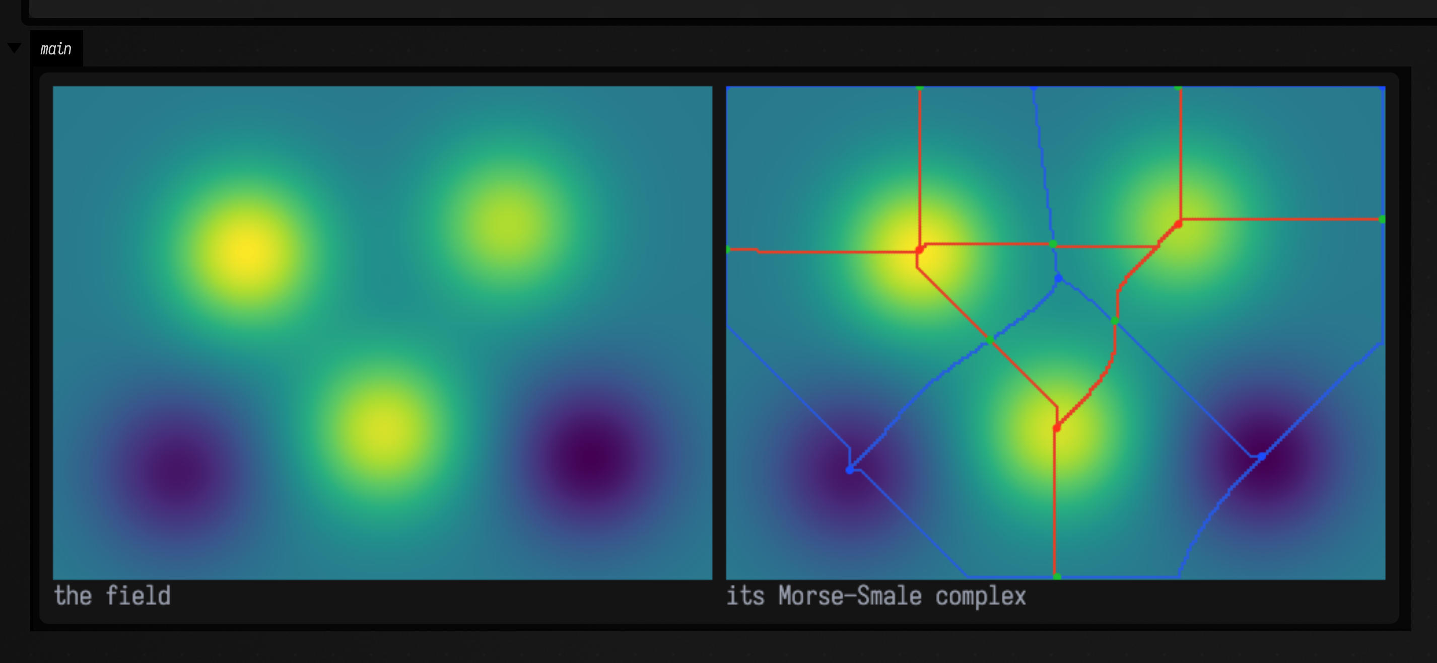
The edge of the grid is part of the landscape. It is lower than the hills and higher than the pits, so some ridges end at the border and some valleys run along it.
result.toFLines() gives one ordinary FLine per separatrix, in pixel coordinates.
criticalPointsFLine() gives one FLine of dots. Img.drawFLines draws FLines over an image, and
Box.lines or anything else that draws FLines can draw them too.
The library is optional
Morse–Smale complexes come from a small native library, field_morse_smale, that Field does
not need in order to run. Build it once with ./gradlew buildMorseSmaleNative; it needs cmake
and a C++ compiler and nothing else. NativeGeometry.describe() says which of Field's native
geometry libraries are present, and calling one that is missing throws an error that says how
to build it.
Persistence: keeping what matters
A real field, whether from noise, a sensor or a photograph, has many tiny hills and pits, and each adds critical points and separatrices. The persistence of a hill is how far you would have to lower it before it merged into a neighbour: its height above the pass that joins it to higher ground. Simplifying at persistence p cancels every pair of critical points whose persistence is below p, and reroutes the separatrices around them, so what remains is the structure that stands out by more than p.
The example below puts noise over the same five bumps. MorseSmale.build computes the complex
once, along with the order in which every pair would cancel. simplify(p) then reads off the
complex at any threshold without recomputing it:
import afield.geometry.topology.morsesmale.*

// The same five bumps, now under fine noise: hundreds of extra hills and pits a pixel or two across.
val bumps = [
    Triple(70.0, 60.0, 1.0),
    Triple(165.0, 50.0, 0.8),
    Triple(120.0, 125.0, 0.9),
    Triple(45.0, 140.0, -0.6),
    Triple(195.0, 135.0, -0.7),
]
val random = java.util.Random(4)
val field =
    Img.generate(240, 180) { x, y ->
            (bumps.sumOf { (cx, cy, a) -> a * exp(-((x - cx).pow(2) + (y - cy).pow(2)) / 900.0) } +
                    0.05 * random.nextGaussian())
                .toFloat()
        }
        .gaussianBlur(1.0)

val complex = MorseSmale.build(field)
val shaded = field.normalized().colormap("viridis")
val panels =
    [0.0, 0.02, 0.3].map { p ->
        val r = complex.simplify(p)
        "persistence $p: ${r.criticalPoints.size} critical points" to
            shaded.drawFLines(r.toFLines() + r.criticalPointsFLine(4.0), scale = 2.0)
    }
showImgGrid(*panels.toTypedArray(), columns = 3, cellSide = 480)
complex.close()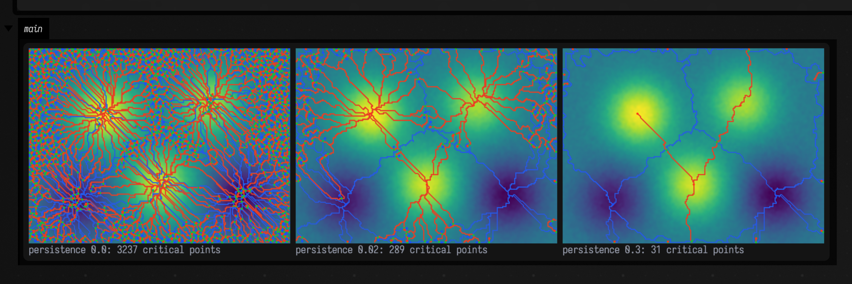
Persistence is measured in the field's own units, so 0.3 here means 0.3 of brightness, height or
whatever the field holds. It is not smoothing. A smoothed field has moved every sample; a
simplified complex has removed features and left the survivors where they were. Blurring first,
as this example does with gaussianBlur(1.0), and then simplifying are different controls, and
both are useful.
complex.survivalCurve() lists, for every threshold where the count changes, how many critical
points survive, which is a quick way to find the threshold where the noise ends.
A photograph
A photograph's brightness is a field like any other. This example crops the leaf print from the living-room photograph on the ONNX page, blurs its brightness slightly, and simplifies at 0.02. The middle panel colours each basin, the region draining to one dark minimum, and draws the valleys that separate them. The right panel draws only the ridges, which follow the bright paper around the leaf and its lobes:
import afield.geometry.topology.morsesmale.*

// The framed leaf print on the left wall of the photograph.
val print = imgFromFile("public/docs/assets/vision/fline-viewer.jpg", 3).crop(78, 262, 128, 236).scaleBy(2.0)
val height = print.luma().gaussianBlur(3.0)

val result = MorseSmale.compute(height, persistence = 0.02)
println(result)

showImgGrid(
    "photograph" to print,
    "basins" to print.overlay(result.segmentationImage(), 0.55).drawFLines(result.toFLines(traceAscending = false)),
    "ridges" to
        print.drawFLines(result.toFLines(traceDescending = false, thickness = 2.0) + result.criticalPointsFLine(5.0)),
    columns = 3,
    cellSide = 320,
)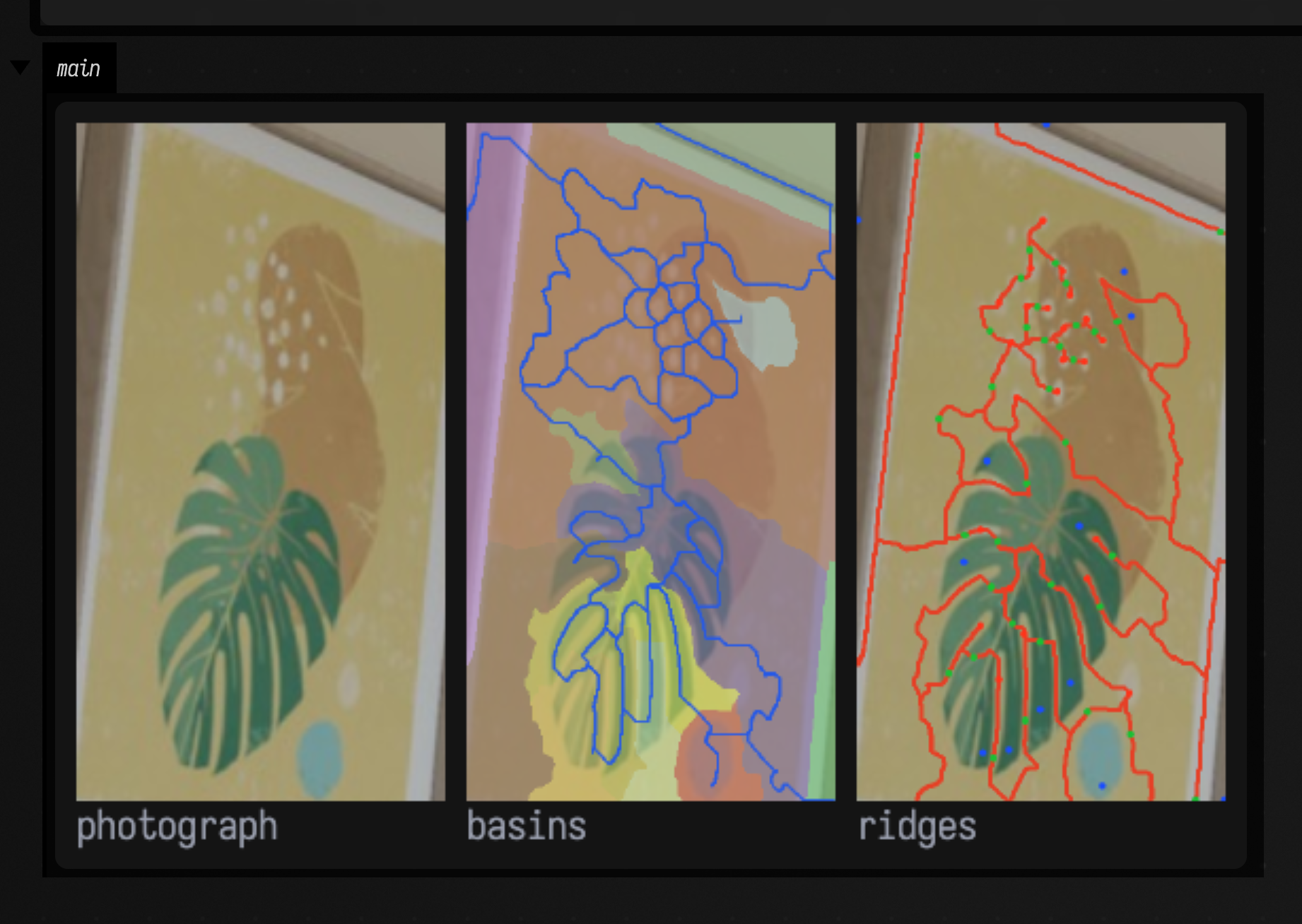
result.basins and result.peaks hold, for every pixel, the id of the minimum or maximum whose
region it is in. segmentationImage() colours them.
Adjusting the threshold live
Building the complex is the expensive step, and simplifying is cheap, so a slider can move the threshold while the box is running. This box builds the complex once and redraws on every slider change:
import afield.geometry.topology.morsesmale.*

val print = imgFromFile("public/docs/assets/vision/fline-viewer.jpg", 3).crop(78, 262, 128, 236).scaleBy(2.0)
val complex = MorseSmale.build(print.luma().gaussianBlur(3.0))

fun show(p: Double) {
    val r = complex.simplify(p)
    showImgGrid(
        "${r.criticalPoints.size} points, ${r.separatrixCount} curves" to
            print.drawFLines(
                r.toFLines(traceDescending = false, thickness = 2.0) + r.criticalPointsFLine(5.0),
                scale = 2.0,
            ),
        channel = "ridges",
        columns = 1,
        cellSide = 520,
    )
}

slider("persistence", min = 0.0, max = 0.3, step = 0.005, initialValue = 0.05) { show(it) }
show(0.05)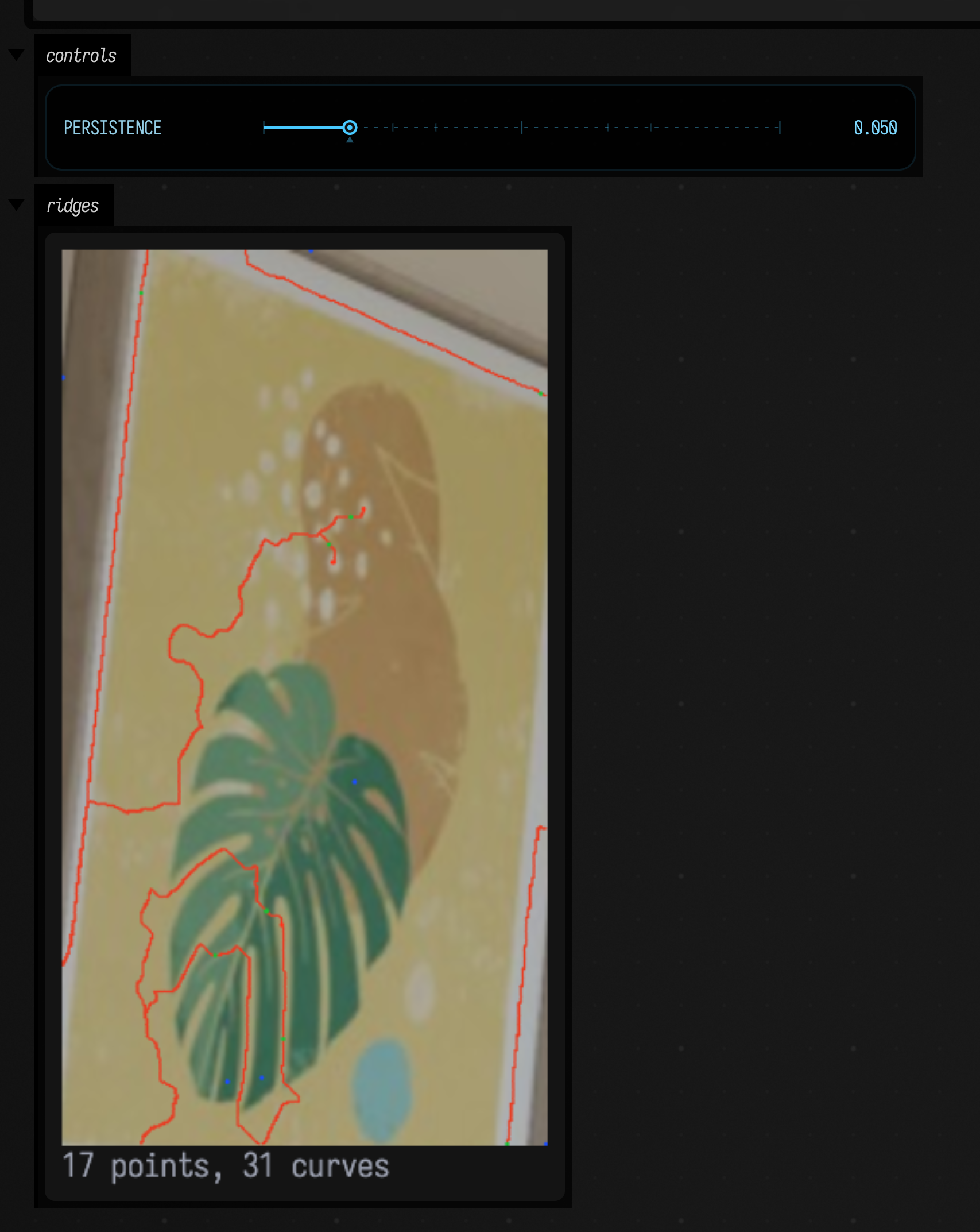
Simplifying a 2048 × 2048 photograph takes about 90 milliseconds on an Apple M-series laptop, against about a second and a half to build its complex. For a field that changes every frame, build on a worker thread, as Running it off the main thread shows.
What the result holds
Everything in a result is ordinary Kotlin data, and nothing is hidden behind the drawing.
result.network is a GeometryNetwork, the common format of Field's geometry-extraction modules:
nodes with typed attribute channels, and curves that name the nodes they join. A curve joins two
nodes only where the complex says it does. Two separatrices that pass through the same pixel do not
share a node.
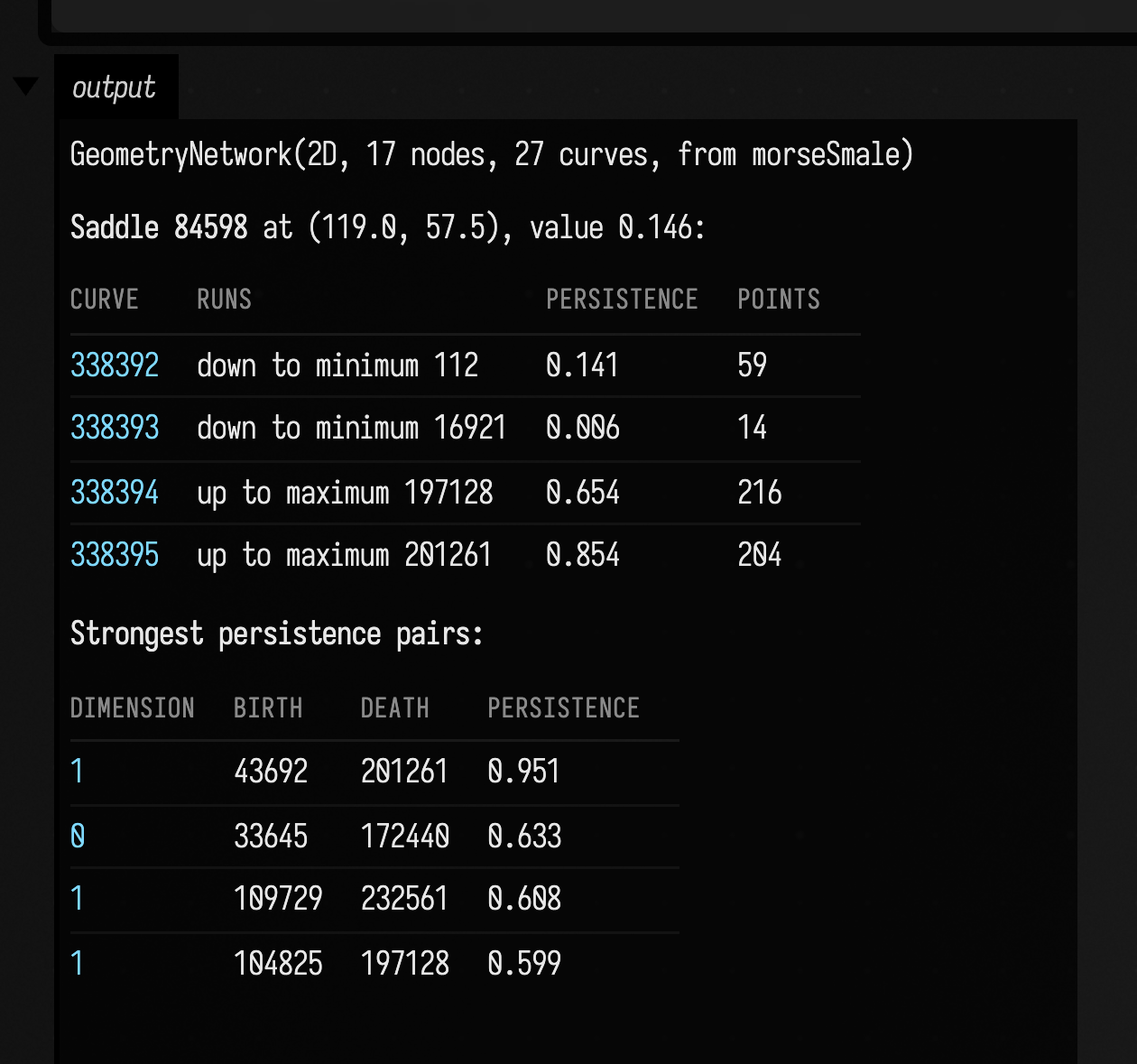
This example walks the network around one saddle and prints the strongest persistence pairs:
import afield.geometry.topology.morsesmale.*

val bumps = [
    Triple(70.0, 60.0, 1.0),
    Triple(165.0, 50.0, 0.8),
    Triple(120.0, 125.0, 0.9),
    Triple(45.0, 140.0, -0.6),
    Triple(195.0, 135.0, -0.7),
]
val field =
    Img.generate(240, 180) { x, y ->
        bumps.sumOf { (cx, cy, a) -> a * exp(-((x - cx).pow(2) + (y - cy).pow(2)) / 900.0) }.toFloat()
    }
val result = MorseSmale.compute(field)
val network = result.network

// The saddle between the two upper hills, and the four separatrices that leave it.
val saddle = result.criticalPoints.filter { it.type == CriticalType.SADDLE }.minBy { abs(it.x - 118) + abs(it.y - 55) }
val arcs =
    network.curvesAt(saddle.id).joinToString("\n") { c ->
        val end = result.complex.critical(c.endNode!!)!!
        "| ${c.id} | ${if (c.attributes["kind"] == 0.0) "down" else "up"} to ${end.type.name.lowercase()} ${end.id} " +
            "| ${c.attributes.getValue("persistence").f3} | ${c.vertexCount} |"
    }

// The persistence diagram, strongest pairs first.
val pairs =
    result.complex.persistencePairs
        .filter { it.death != null }
        .sortedByDescending { it.persistence }
        .take(4)
        .joinToString("\n") { "| ${it.dimension} | ${it.birth} | ${it.death} | ${it.persistence.f3} |" }

markdown(
    """
$network

**Saddle ${saddle.id}** at (${saddle.x.f1}, ${saddle.y.f1}), value ${saddle.value.f3}:

| curve | runs | persistence | points |
| --- | --- | ---: | ---: |
$arcs

**Strongest persistence pairs:**

| dimension | birth | death | persistence |
| ---: | ---: | ---: | ---: |
$pairs
""",
)
The parts of a result:
criticalPoints |
the survivors at this threshold. Each has an id, type, value, x, y and cancelledAt, the threshold that would remove it. |
network |
the complex as a GeometryNetwork. Node channels: type (0 minimum, 1 saddle, 2 maximum), value, cancelledAt. Curve attributes: kind (0 descending, 1 ascending), persistence, saddleValue, extremumValue. Each curve also has the field's value at every vertex, as the sample value. |
basins, peaks |
per pixel, the id of the region's minimum or maximum. A pixel whose uphill path leaves the grid has peak -1. |
descending, ascending |
the network with only one kind of separatrix. |
toFLines(...) |
the separatrices as FLines, each carrying curveId, startNode, endNode and the whole network as geometryNetwork. smooth = true draws each as a spline through the same points; the topology does not change. |
complex.persistencePairs |
the persistence diagram: dimension 0 pairs a minimum with the saddle that merges it away, dimension 1 a saddle with a maximum. |
complex.cancellations |
every cancellation, in order, with its persistence. |
complex.timings |
milliseconds spent on each stage of the build. |
Ids are grid cells, so a critical point keeps its id across thresholds, and across recomputation of a changing field for as long as it stays on the same cell. A separatrix keeps its id for as long as both its ends survive. Animations and other objects can be keyed to them.
Running it off the main thread
MorseSmale.computeAsync and MorseSmale.buildAsync do the work on a worker thread and return a
CompletableFuture, which is what runAsync takes. The box stays responsive while a large field is
analysed, and the result is shown when it arrives:
import afield.geometry.topology.morsesmale.*

val photo = imgFromFile("public/docs/assets/vision/fline-viewer.jpg", 3)
runAsync(
    onResult = { r: MorseSmaleResult ->
        showImgGrid("ridges" to photo.drawFLines(r.toFLines(traceDescending = false)), columns = 1, cellSide = 800)
    },
) {
    MorseSmale.computeAsync(photo.luma().gaussianBlur(2.0), persistence = 0.05)
}
A MorseSmaleComplex holds native memory until it is closed. compute closes its own. A complex
that build makes while a box runs is closed when the box runs again, and stays open after a stop
so that a slider still works. One made on a worker thread, as buildAsync does, is yours to close.
How the complex is computed
The grid is cut into triangles, each square split along the same diagonal. On that mesh the library builds the discrete gradient of the field, a pairing of each vertex, edge and triangle with a neighbour that it flows into. This is Forman's discrete Morse theory, built with the lower-star algorithm of Robins, Wood and Sheppard. The cells left unpaired are the critical points: a minimum is a vertex, a saddle an edge, a maximum a triangle. That is why saddles sit on edge midpoints and maxima on triangle centres. Separatrices follow the pairing from each saddle. Ties between equal samples are broken by pixel index, so a flat region always produces the same answer, though the answer depends on that rule.
Simplification follows Gyulassy, Natarajan, Pascucci and Hamann (2008). A saddle and an extremum joined by exactly one separatrix are removed together, and every other separatrix that reached the extremum is rerouted through the saddle. The library computes the whole sequence once, in order of persistence, and a threshold replays part of it. Outside the grid is treated as one maximum higher than everything, so peaks next to the border can be removed like any other. Simplification stops at a saddle that is joined to the same extremum twice, because removing it would change the topology, so a fully simplified complex can keep a few such pairs. The persistence diagram is computed separately and always pairs every critical point.
How this is checked
The native test (native/field-morse-smale/tests/) checks that minima minus saddles plus maxima
is exactly 1, as it must be for a disc, at every threshold, and that the persistence pairs
cover every critical point once. tools/validate_morse_smale.py compares the persistence
diagram with gudhi 3.13 and with TTK 1.3.0, the Topology ToolKit, on noise, saddles, a monkey
saddle and a gradient-magnitude field; the pairs agree exactly in both dimensions. TTK splits
the grid's squares along the other diagonal, so the script flips the field vertically before
handing it over. Without the flip the diagrams differ, which is how we know the triangulation
matters. MorseSmaleBenchmark times each stage at 512², 1024² and 2048².