Boolean networks to FLine examples
A Boolean network is a set of nodes that are each on or off, plus a rule that computes every node's next value from the current values of the others. Because there are only finitely many states, every run ends up in a loop or at a fixed point (an attractor), and Field can list them all exactly. Each example below draws the network's wiring next to what it does over time.
Wiring and state-space, side by side
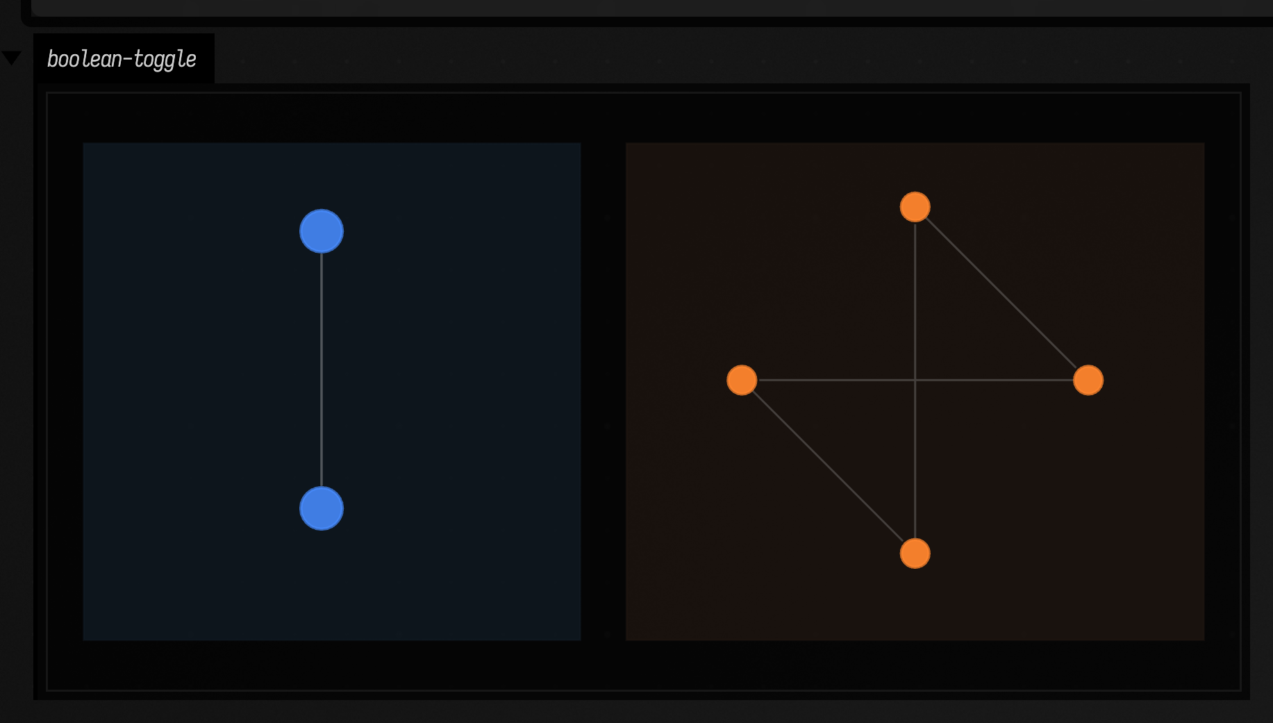
toggleNetwork() is two nodes, A = NOT B and B = A, and that is already enough to separate the two views the rest of the page relies on: the causal wiring graph, which has one arrow per dependency, and the induced state-transition graph, which has one arrow per state.
:::static
val net = toggleNetwork()
val attrs = net.findAttractors()

:::fold helpers: offset a drawing, fill a background panel
fun shift(lines: List<FLine>, dx: Double, dy: Double) = lines.map { it + vec(dx, dy, 0) }

fun panel(x: Double, y: Double, w: Double, h: Double, color: Vec4) = fline {
    rect(x, y, w, h)
    filled = true
    stroked = true
    thickness = 1.0
    this.color = color
}

:::endfold

lines(
    [
        panel(30.0, 40.0, 430.0, 430.0, vec(0.08, 0.13, 0.18, 0.56)),
        panel(500.0, 40.0, 500.0, 430.0, vec(0.16, 0.11, 0.08, 0.54)),
    ] +
        shift(net.drawNetworkGraph(radius = 120.0, nodeR = 18.0), 80.0, 80.0) +
        shift(net.drawStateTransitionGraph(radius = 150.0), 560.0, 55.0),
    channel = "boolean-toggle",
    w = 1060.0,
    h = 520.0,
    fitToSize = true,
)
The left image tells you what depends on what; the right image tells you what that dependency does to every possible state. Here the two coincide: with four states and both nodes reading the other, the whole state space is a single period-4 loop, 00 -> 10 -> 11 -> 01 and back.
Segment-polarity basins and a transient
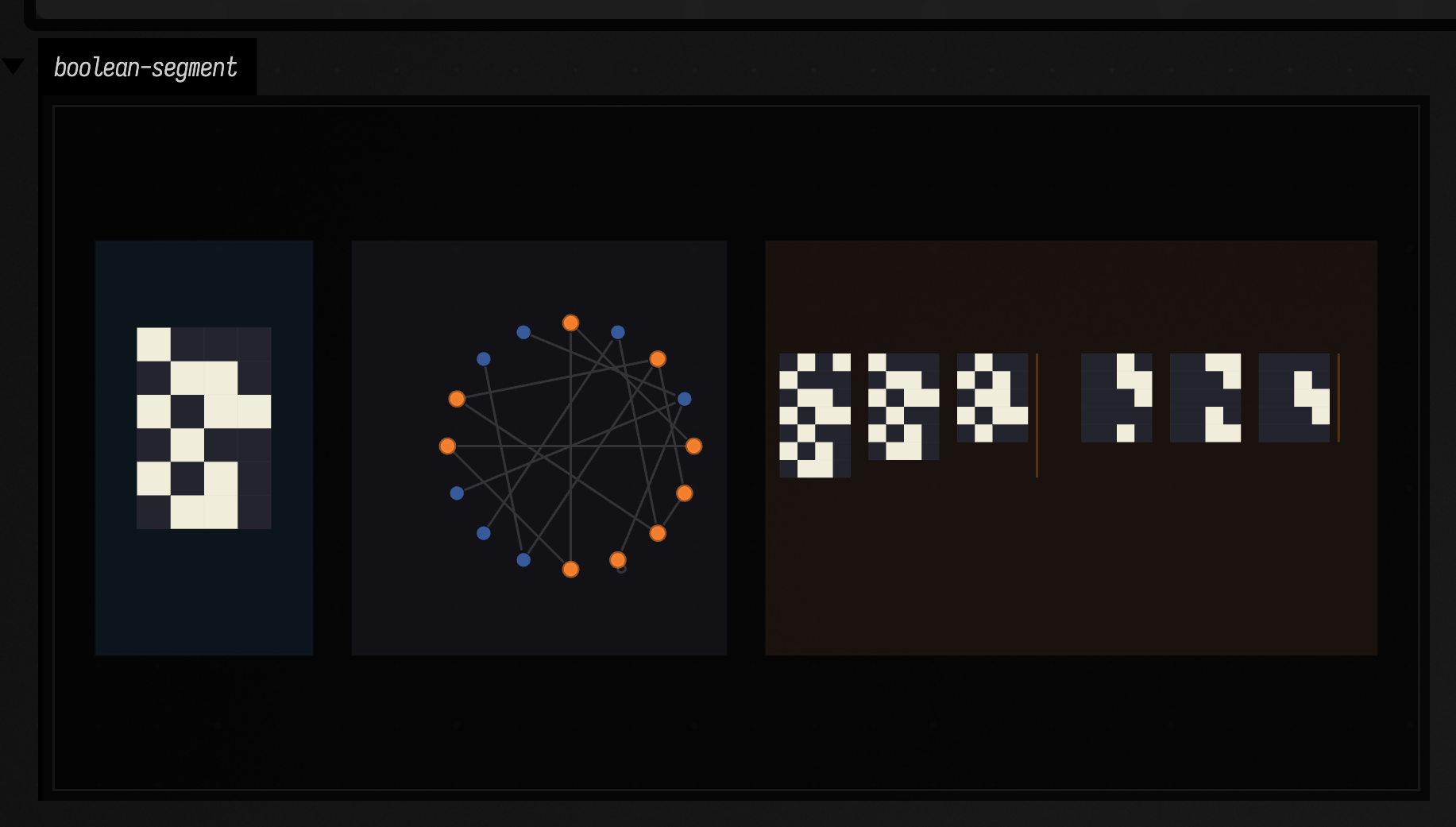
segmentPolarityNetwork() has four nodes, so sixteen states, and unlike the toggle it does not spend all of them on one cycle. There is more than one attractor, so there is more than one basin: the set of starting states that end on a given attractor.
:::static
val net = segmentPolarityNetwork()
val attrs = net.findAttractors().sortedByDescending { it.basin.size }
val largest = attrs.first()
val cycleStates = largest.cycle.map { net.stateToInt(it) }.toSet()
val start = largest.basin.firstOrNull { it !in cycleStates } ?: largest.basin.first()
val trajectory = net.trajectoryUntilCycle(net.intToState(start))
val shown = attrs.take(2)

:::fold helpers: offset a drawing, fill a background panel
fun shift(lines: List<FLine>, dx: Double, dy: Double) = lines.map { it + vec(dx, dy, 0) }

fun panel(x: Double, y: Double, w: Double, h: Double, color: Vec4) = fline {
    rect(x, y, w, h)
    filled = true
    stroked = true
    thickness = 1.0
    this.color = color
}

:::endfold

lines(
    [
        panel(30.0, 40.0, 220.0, 420.0, vec(0.08, 0.13, 0.18, 0.56)),
        panel(290.0, 40.0, 380.0, 420.0, vec(0.10, 0.10, 0.14, 0.56)),
        panel(710.0, 40.0, 620.0, 420.0, vec(0.16, 0.11, 0.08, 0.54)),
    ] +
        shift(net.drawUnrolled(trajectory, cellSize = 34.0), 72.0, 128.0) +
        shift(net.drawStateTransitionGraph(radius = 125.0), 347.0, 83.0) +
        shift(net.drawAttractorBasins(shown, samplesPerAttractor = 3, cellSize = 18.0), 724.0, 154.0),
    channel = "boolean-segment",
    w = 1360.0,
    h = 520.0,
    fitToSize = true,
)
The left panel is one concrete transient, the middle panel is the whole 16-state transition graph, and the right panel samples the two largest basins as miniature spacetime strips. The transient is the path from a starting state to its attractor: which of the sixteen states you start from decides which attractor you end on, and how many steps it takes.
Random Kauffman regimes as a plotted sweep
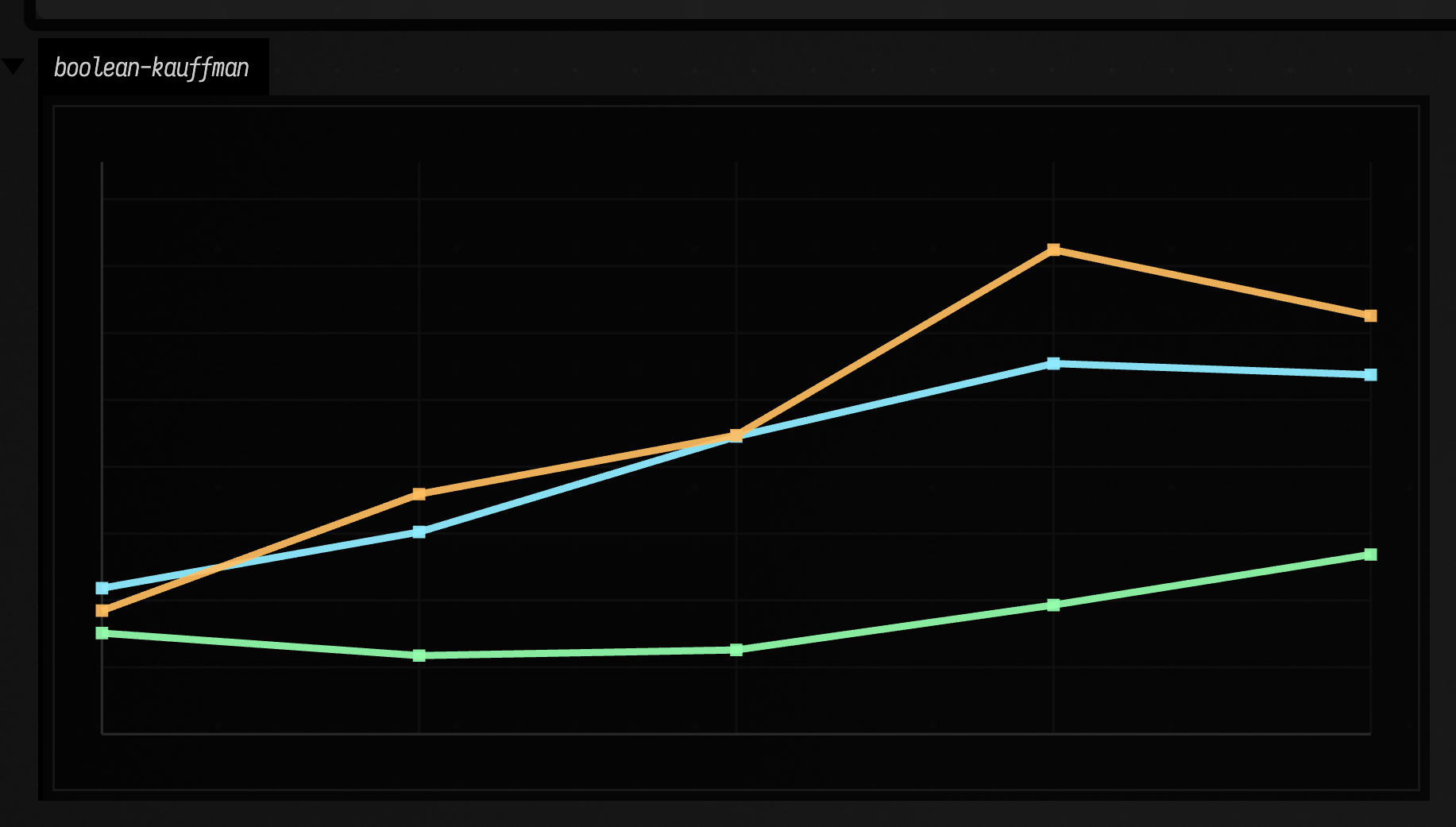
The two networks above were hand-made. This one asks a population question instead: as in-degree k rises in random N-K Kauffman systems, what happens to the typical attractor count and period?
:::static
data class SweepRow(val k: Int, val attractors: Double, val period: Double, val fixed: Double)

val rows =
    (1..5).map { k ->
        val runs =
            (0 until 18).map { seed ->
                val attrs = kauffmanNetwork(n = 8, k = k, seed = seed.toLong()).findAttractors()
                Triple(
                    attrs.size.toDouble(),
                    if (attrs.isEmpty()) 0.0 else attrs.map { it.period.toDouble() }.average(),
                    attrs.count { it.period == 1 }.toDouble(),
                )
            }
        SweepRow(
            k = k,
            attractors = runs.map { it.first }.average(),
            period = runs.map { it.second }.average(),
            fixed = runs.map { it.third }.average(),
        )
    }

:::fold plot helpers: shared y scale, axes and grid, polylines, square markers
val maxY =
    [
            rows.maxOf { it.attractors },
            rows.maxOf { it.period },
            rows.maxOf { it.fixed },
        ]
        .max() + 0.5

fun guides() = [
    fline {
        moveTo(80, 580)
        lineTo(1100, 580)
        moveTo(80, 120)
        lineTo(80, 580)
        color = vec(1, 1, 1, 0.22)
        thickness = 1.1
    },
    fline {
        for (i in 0..8) {
            val y = 580.0 - i / 8.0 * 430.0
            moveTo(80, y)
            lineTo(1100, y)
        }
        for (i in rows.indices) {
            val x = 80.0 + i.toDouble() / (rows.size - 1).coerceAtLeast(1).toDouble() * 1020.0
            moveTo(x, 120.0)
            lineTo(x, 580.0)
        }
        color = vec(1, 1, 1, 0.08)
        thickness = 1.0
    },
]

fun curve(values: List<Double>, color: Vec4, thickness: Double): FLine = fline {
    breakNext()
    values.forEachIndexed { i, value ->
        val x = 80.0 + i.toDouble() / (values.size - 1).coerceAtLeast(1).toDouble() * 1020.0
        val y = 580.0 - value / maxY * 430.0
        lineTo(x, y)
    }
    this.color = color
    this.thickness = thickness
}

fun markers(values: List<Double>, color: Vec4, size: Double): FLine = fline {
    filled = true
    stroked = false
    values.forEachIndexed { i, value ->
        val x = 80.0 + i.toDouble() / (values.size - 1).coerceAtLeast(1).toDouble() * 1020.0
        val y = 580.0 - value / maxY * 430.0
        rect(x - size, y - size, 2 * size, 2 * size)
    }
    this.color = color
}

:::endfold

lines(
    guides() +
        listOf(
            curve(rows.map { it.attractors }, vec(0.56, 0.92, 1.0, 0.95), 3.0),
            curve(rows.map { it.period }, vec(1.0, 0.74, 0.38, 0.92), 3.0),
            curve(rows.map { it.fixed }, vec(0.58, 1.0, 0.68, 0.92), 3.0),
            markers(rows.map { it.attractors }, vec(0.56, 0.92, 1.0, 0.95), 5.0),
            markers(rows.map { it.period }, vec(1.0, 0.74, 0.38, 0.92), 5.0),
            markers(rows.map { it.fixed }, vec(0.58, 1.0, 0.68, 0.92), 5.0),
        ),
    channel = "boolean-kauffman",
    w = 1180.0,
    h = 660.0,
    fitToSize = true,
)
The plot has no legend, so: blue is the mean number of attractors, orange the mean period, green the mean number of fixed points, each averaged over 18 seeds at n = 8 for k from 1 to 5, and all three share one y scale. All three rise with k: more connections give more attractors and longer ones. Orange overtakes blue around the middle of the sweep and turns down at k = 5, and green stays under blue throughout, as it has to: a fixed point is a period-1 attractor and so is counted in both.
Boolean attractors as drum grids
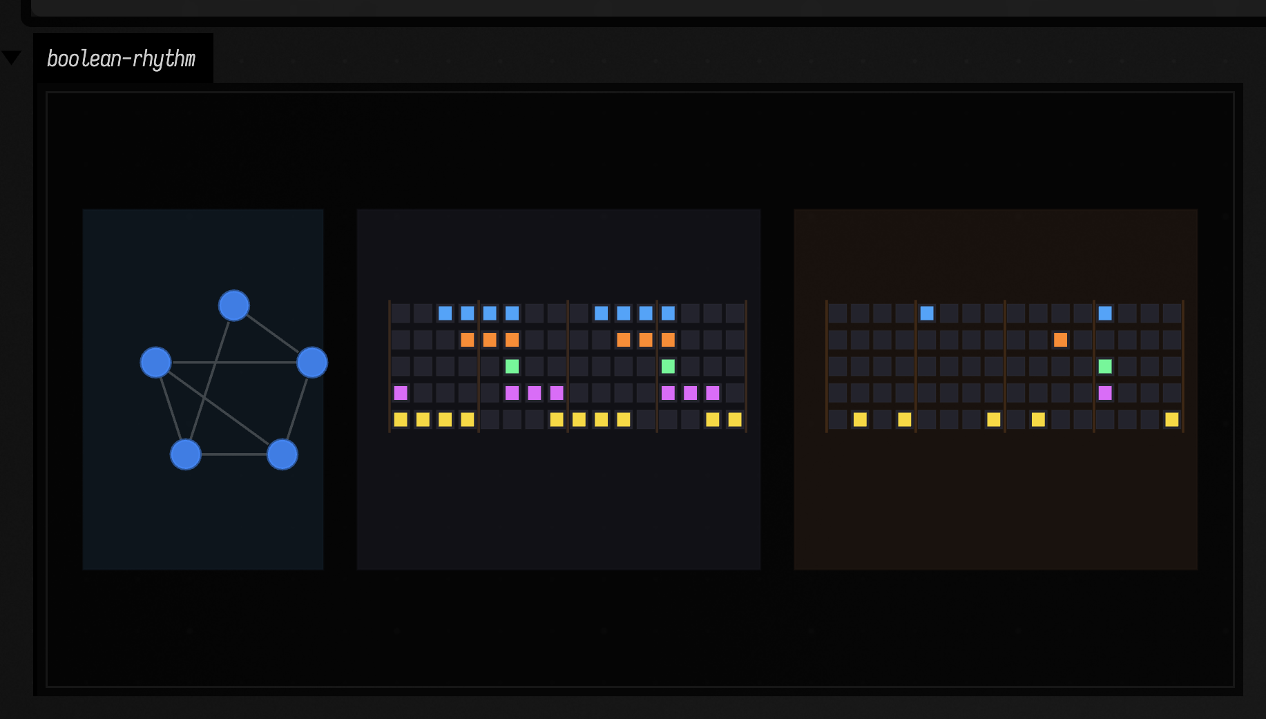
A limit cycle repeats on a fixed period, so it is already a rhythm. You can treat each node as a lane directly, or gate the cycle with a beat phase such as step % 4 and turn the same binary motion into kick / snare / hat style triggers.
:::static
data class RhythmCandidate(val seed: Int, val net: BooleanNetwork, val attr: Attractor, val score: Double)

fun activity(attr: Attractor, net: BooleanNetwork): Double =
    attr.cycle.sumOf { state -> state.count { it } }.toDouble() / (attr.period * net.size).toDouble()

val candidate =
    (0..240)
        .mapNotNull { seed ->
            val net = kauffmanNetwork(n = 5, k = 2, seed = seed.toLong())
            net.findAttractors()
                .filter { it.period in 5..10 }
                .map { attr ->
                    val density = activity(attr, net)
                    val periodScore = 1.0 - kotlin.math.abs(attr.period - 8) / 8.0
                    val densityScore = 1.0 - kotlin.math.abs(density - 0.42)
                    val basinScore = attr.basin.size.toDouble() / (1 shl net.size).toDouble()
                    RhythmCandidate(seed, net, attr, periodScore * 1.6 + densityScore * 1.2 + basinScore)
                }
                .maxByOrNull { it.score }
        }
        .maxByOrNull { it.score }!!

val natural = candidate.attr.repeatedCycle(16)
val gated = natural.mapIndexed { step, state ->
    booleanArrayOf(
        state[0] && step % 4 == 0,
        state[1] && step % 4 == 2,
        state[2] && step % 2 == 0,
        state[3] && (step % 8 == 4 || step % 8 == 12),
        state[4] && (step % 4 == 1 || step % 4 == 3),
    )
}

:::fold helpers: offset a drawing, fill a background panel
fun shift(lines: List<FLine>, dx: Double, dy: Double) = lines.map { it + vec(dx, dy, 0) }

fun panel(x: Double, y: Double, w: Double, h: Double, color: Vec4) = fline {
    rect(x, y, w, h)
    filled = true
    stroked = true
    thickness = 1.0
    this.color = color
}

:::endfold

lines(
    [
        panel(30.0, 40.0, 280.0, 420.0, vec(0.08, 0.13, 0.18, 0.56)),
        panel(350.0, 40.0, 470.0, 420.0, vec(0.10, 0.10, 0.14, 0.56)),
        panel(860.0, 40.0, 470.0, 420.0, vec(0.16, 0.11, 0.08, 0.54)),
    ] +
        shift(candidate.net.drawNetworkGraph(radius = 96.0, nodeR = 17.0), 76.0, 118.0) +
        shift(
            drawRhythmGrid(natural, cellW = 21.0, cellH = 22.0, stepGap = 5.0, laneGap = 9.0, accentEvery = 4),
            390.0,
            150.0,
        ) +
        shift(
            drawRhythmGrid(gated, cellW = 21.0, cellH = 22.0, stepGap = 5.0, laneGap = 9.0, accentEvery = 4),
            900.0,
            150.0,
        ),
    channel = "boolean-rhythm",
    w = 1380.0,
    h = 520.0,
    fitToSize = true,
)
The middle grid is the raw attractor repeated over two bars. The right grid is the same cycle clock-gated into five kick / snare / hat / clap / percussion lanes, ready to hand to a sampler. The grids repeat exactly, so you can read them off the page.
Here is the right-hand grid played through Field's Dirt-Samples, eight steps a second, kick, snare,
hat, clap and percussion lanes as bd, sn, hh, cp and perc. The 16 steps play twice:
For the next step, where those grids become NoteProcess objects and live Dirt triggers, continue with Boolean network music examples. For related work where static structure and measured behavior are plotted together, continue with Values over time (interpolants, keyframes, correlations & estimation) and Sorting networks examples.
The public declarations used on this page are listed, with their KDoc, in the codebase reference: booleannetworks.kt. Start from what's already in the box.