Principal curves: smooth curves through point clouds

A principal curve runs through the middle of a cloud of points, the way a pen line runs down the middle of a smudged stroke. Fit one to a scatter and you can inspect the resulting curve and how widely the points spread along its length. A collection of such curves, some of them branching, is a principal forest.

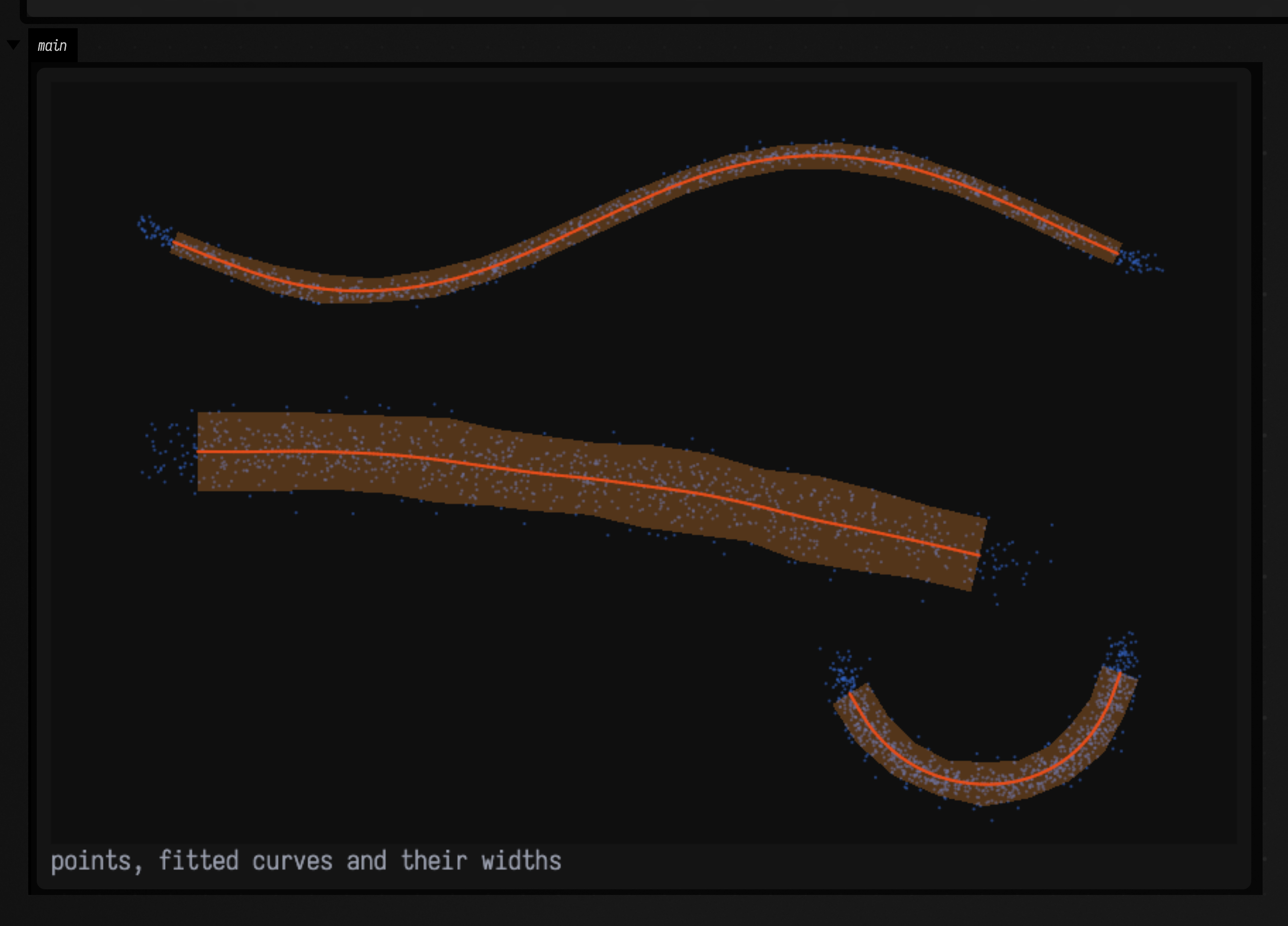
The points can come from anywhere: a photograph's dark pixels, a stipple, a particle system, a depth map, or a box that generated them. They need not form visible lines. This example scatters 1000 points around each of three strands of different thickness, then fits three curves. widthFLines() draws a band two standard deviations of the scatter to each side, so the bands show which strand was drawn with the broader pen:

import afield.geometry.curves.principal.*

// Three noisy strands of different thickness, 1000 points each.
val random = java.util.Random(2)
val points = DoubleArray(3000 * 2)
for (i in 0 until 3000) {
    val t = random.nextDouble()
    val (x, y, spread) = when (i % 3) {
        0 -> Triple(30 + 360 * t, 50 + 25 * sin(7 * t), 2.0)
        1 -> Triple(40 + 300 * t, 130 + 40 * t * t, 7.0)
        else -> Triple(330 + 50 * cos(3 * t), 200 + 50 * sin(3 * t), 3.5)
    }
    points[2 * i] = x + spread * random.nextGaussian()
    points[2 * i + 1] = y + spread * random.nextGaussian()
}

val forest = PrincipalCurves.fit(points, curves = 3, nodes = 45)

val canvas = Img(420, 270, 3, FloatArray(420 * 270 * 3) { 0.06f })
showImgGrid(
    "points, fitted curves and their widths" to
        canvas.drawFLines(
            [forest.pointsFLine(pointSize = 2.0)] + forest.widthFLines() + forest.toFLines(),
            scale = 2.0,
        ),
    columns = 1,
    cellSide = 840,
)

PrincipalCurves.fit takes the points as a flat array (x, y, x, y, … or x, y, z, … with dimension = 3), optional per-point weights, how many separate curves to start with, and how many nodes to use in all. It returns a PrincipalForest. toFLines() draws the curves as smooth splines through the forest's nodes, and pointsFLine() draws the input points.

A fitted curve stops a little inside its last points, by about half the spacing between its nodes. More nodes bring the ends closer.

Width and uncertainty are different things

nodeStatistics() reports, for every node, statistics of the points that project near it:

• width: the standard deviation of the points across the curve, i.e. how spread out the data is;
• standard error: how precisely the node's own position is known from those points;
• support: the total weight of the points near the node;
• effective sample size (nEff): how many equally weighted points would locate the node as well. A point is shared between the two nodes of its edge, so many partly shared points can make nEff larger than support.

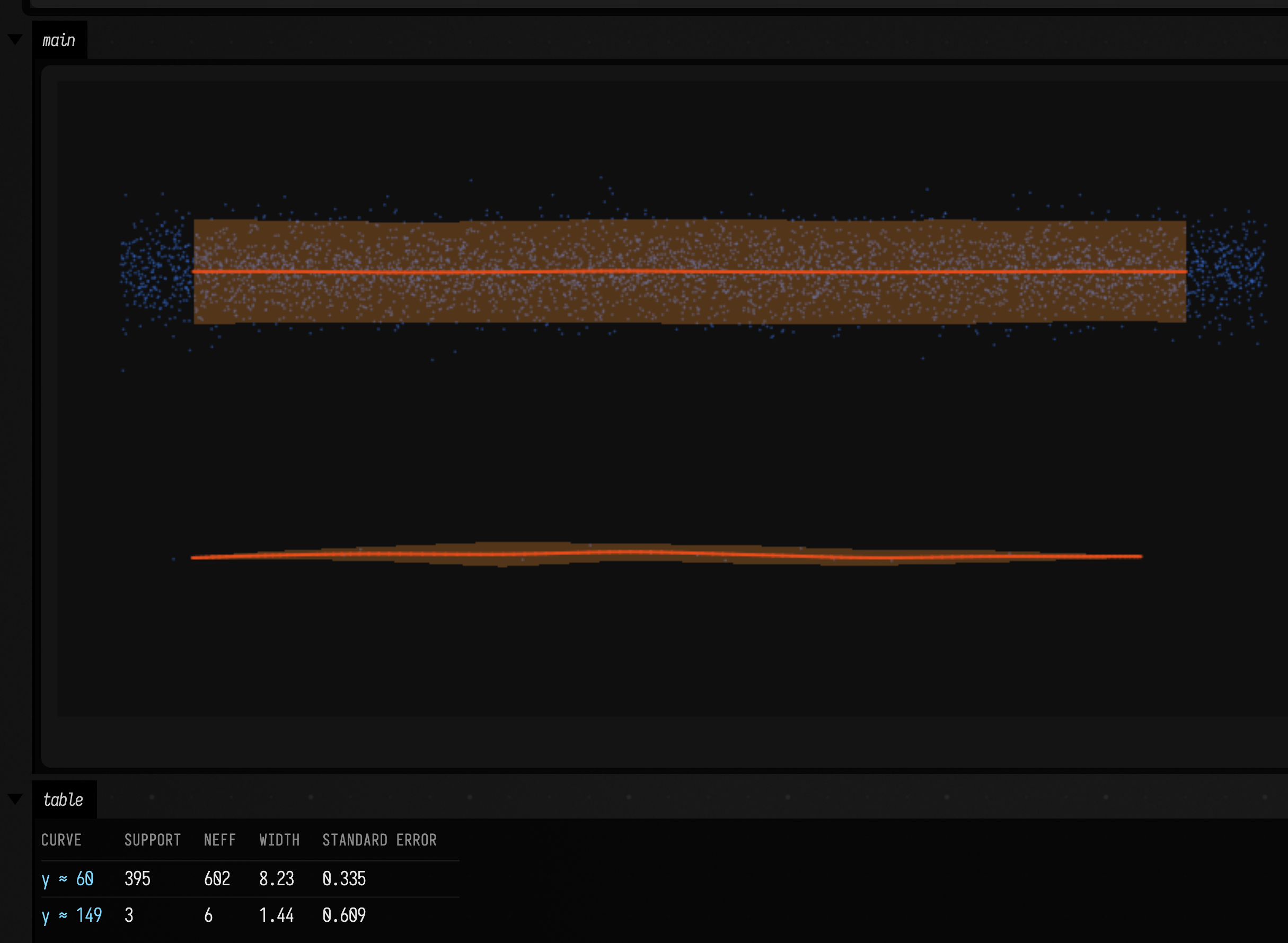
A broad scatter of many points has a large width but is located precisely. A thin line of very few points has a small width but an uncertain position. This example fits one of each and prints both numbers for a node in the middle of each curve. Each curve gets the same ten nodes, so the thin one has fewer than two points per node. The thin strand comes out six times narrower and its nodes about twice as uncertain:

import afield.geometry.curves.principal.*

val random = java.util.Random(9)
// 4000 points spread 8 pixels either side of y = 60; 16 points spread 1.5 pixels around y = 150.
val broad = (0 until 4000).flatMap { [20 + 360 * random.nextDouble(), 60 + 8 * random.nextGaussian()] }
val thin = (0 until 16).flatMap { [20 + 360 * random.nextDouble(), 150 + 1.5 * random.nextGaussian()] }
val points = (broad + thin).toDoubleArray()

// Ten nodes on each curve, started from two strokes, fitted without growing.
val forest = PrincipalCurves.create(points)
forest.initFromFLines(
    [FLine().moveTo(30, 60).lineTo(370, 60), FLine().moveTo(30, 150).lineTo(370, 150)],
    nodesPerCurve = 10,
)
forest.fit()
val stats = forest.nodeStatistics()
val rows =
    forest.network.curves.joinToString("\n") { c ->
        val i = c.samples.getValue("graphNode")[c.vertexCount / 2].toInt()
        "| y ≈ ${c.vertex(c.vertexCount / 2).y.f0} | ${stats.support[i].f0} | ${stats.nEff[i].f0} | ${stats.width[i].f2} | ${stats.standardError[i].f3} |"
    }

val canvas = Img(400, 200, 3, FloatArray(400 * 200 * 3) { 0.06f })
showImgGrid(
    "" to canvas.drawFLines([forest.pointsFLine(1.5)] + forest.widthFLines() + forest.toFLines(), scale = 2.0),
    columns = 1,
    cellSide = 800,
)
markdown(
    "table",
    """
| curve | support | nEff | width | standard error |
| --- | ---: | ---: | ---: | ---: |
$rows
""",
)

In 3D, a node has a 2 × 2 covariance in the plane across the curve instead of a single variance, so a flattened tube of points gives an elliptical cross-section. nodeStatistics().spread holds the covariance and basis holds the two directions it is measured in. The covariance sample on each curve of network holds the same values.

Trees, and points from a photograph

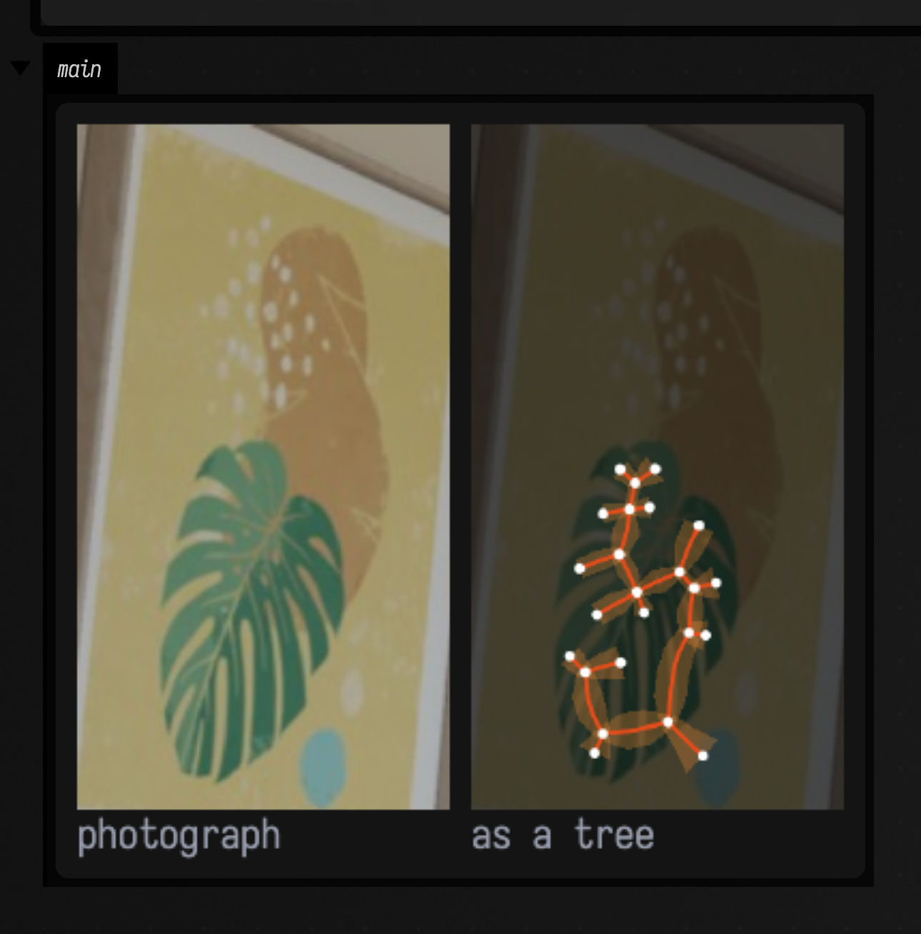
With allowBranching = true a forest can grow branches, and each component becomes a tree. Points can carry weights. This example takes every pixel of the leaf print that is greener than it is red or blue, weights it by how much greener, and fits a tree of 40 nodes:

import afield.geometry.curves.principal.*

// The leaf in the print, as points: every pixel greener than it is red or blue, weighted by how much.
val print = imgFromFile("public/docs/assets/vision/fline-viewer.jpg", 3).crop(78, 262, 128, 236).scaleBy(2.0)
val points = ArrayList<Double>()
val weights = ArrayList<Double>()
for (y in 0 until print.height) for (x in 0 until print.width) {
    val green = print.at(x, y, 1) - maxOf(print.at(x, y, 0), print.at(x, y, 2))
    if (green > 0.04) {
        points.add(x.toDouble())
        points.add(y.toDouble())
        weights.add(green.toDouble())
    }
}

val forest =
    PrincipalCurves.fit(points.toDoubleArray(), weights = weights.toDoubleArray(), nodes = 40, allowBranching = true)
val junctions = forest.network.nodesFLine().also {
    it.pointed = true
    it.pointSize = 7.0
    it.color = Vec4(1f, 1f, 1f, 1f)
}

val dark = Img(print.width, print.height, 3, FloatArray(print.width * print.height * 3))
showImgGrid(
    "photograph" to print,
    "as a tree" to
        print.overlay(dark, 0.6).drawFLines(forest.widthFLines(1.0) + forest.toFLines(thickness = 2.5) + junctions),
    columns = 2,
    cellSide = 320,
)

forest.network is the forest as a GeometryNetwork, the format Field's geometry-extraction modules share. Its nodes are the branch points and tips, its curves are the stretches between them, and every curve vertex carries width, support, nEff, residual and standardError samples.

Crossing or branching: who decides

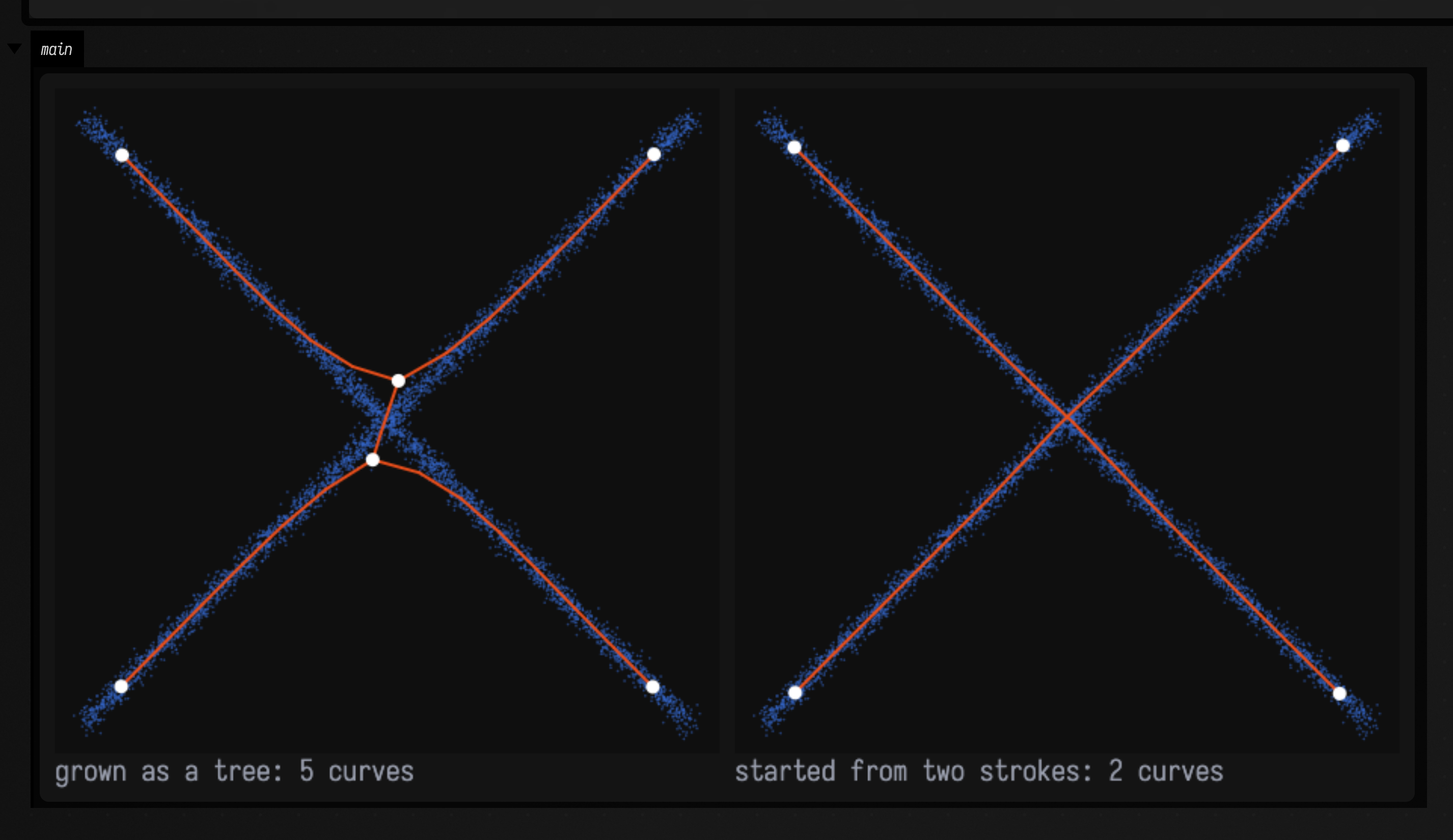
Two strokes that cross look the same as four branches meeting at a point, if all you have are the points. A tree grown from nothing takes the second reading, because a junction is the cheapest way for one connected graph to cover both strokes. To keep a crossing a crossing, start the forest from the strokes you mean and grow it as curves only. Separate curves never share a node, so they pass over each other:

import afield.geometry.curves.principal.*

// Two straight strokes that cross, as 6000 points.
val random = java.util.Random(5)
val points = DoubleArray(6000 * 2)
for (i in 0 until 6000) {
    val t = random.nextDouble() * 200 - 100
    points[2 * i] = 110 + t + 2 * random.nextGaussian()
    points[2 * i + 1] = 110 + (if (i % 2 == 0) t else -t) + 2 * random.nextGaussian()
}

// Grown from nothing as a tree, versus started from the two strokes and grown as curves.
val grown = PrincipalCurves.fit(points, nodes = 30, allowBranching = true)
val strokes = [FLine().moveTo(20, 20).lineTo(200, 200), FLine().moveTo(20, 200).lineTo(200, 20)]
val drawn = PrincipalCurves.fit(points, nodes = 30, from = strokes)

val canvas = Img(220, 220, 3, FloatArray(220 * 220 * 3) { 0.06f })
fun picture(f: PrincipalForest) = canvas.drawFLines(
    [f.pointsFLine(1.5)] +
        f.toFLines(smooth = false) +
        f.network.nodesFLine().also {
            it.pointed = true
            it.pointSize = 9.0
            it.color = Vec4(1f, 1f, 1f, 1f)
        },
    scale = 2.0,
)
showImgGrid(
    "grown as a tree: ${grown.network.curves.size} curves" to picture(grown),
    "started from two strokes: ${drawn.network.curves.size} curves" to picture(drawn),
    columns = 2,
    cellSide = 440,
)

from takes any FLines, so a few rough strokes drawn on the canvas can be fitted onto a point cloud. Each subpath becomes one curve, and a closed subpath becomes a loop.

Stiffness, live

Two numbers set the character of the fit. lambda penalises stretching, so a larger value gives a shorter, tauter graph. mu penalises bending at every node with two or more neighbours, so a larger value gives smoother curves. Both are passed as ElasticParameters. Fitting a few thousand points takes a fraction of a second, so a slider can refit as you drag:

import afield.geometry.curves.principal.*

val random = java.util.Random(2)
val points = DoubleArray(3000 * 2)
for (i in 0 until 3000) {
    val t = random.nextDouble()
    val (x, y, spread) = when (i % 3) {
        0 -> Triple(30 + 360 * t, 50 + 25 * sin(7 * t), 2.0)
        1 -> Triple(40 + 300 * t, 130 + 40 * t * t, 7.0)
        else -> Triple(330 + 50 * cos(3 * t), 200 + 50 * sin(3 * t), 3.5)
    }
    points[2 * i] = x + spread * random.nextGaussian()
    points[2 * i + 1] = y + spread * random.nextGaussian()
}
val canvas = Img(420, 270, 3, FloatArray(420 * 270 * 3) { 0.06f })

fun show(mu: Double) {
    val forest = PrincipalCurves.fit(points, curves = 3, nodes = 45, parameters = ElasticParameters(mu = mu))
    showImgGrid(
        "mu = $mu" to
            canvas.drawFLines([forest.pointsFLine(2.0)] + forest.widthFLines() + forest.toFLines(), scale = 2.0),
        channel = "fit",
        columns = 1,
        cellSide = 520,
    )
    forest.close()
}

slider("bending (mu)", min = 0.0, max = 2.0, step = 0.05, initialValue = 0.1) { show(it) }
show(0.1)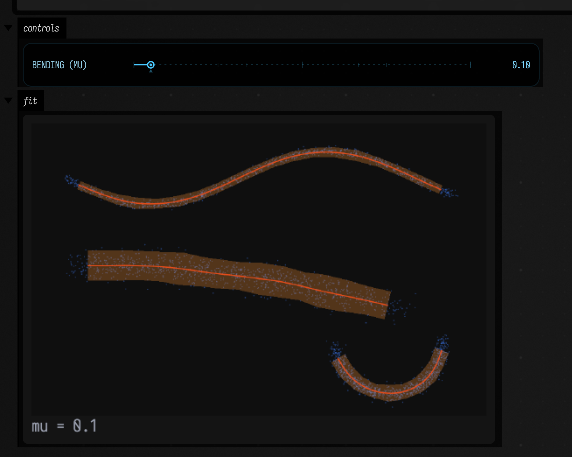

Editing a fitted forest

A PrincipalForest keeps its state between calls, so it can be changed and refitted without starting again:

ElasticParameters(trimmingRadius = r) makes the fit ignore points farther than r from every node, so a few stray points do not drag a curve off its strand.

A forest made in a box is closed when the box runs again; one made with PrincipalCurves.fitAsync on a worker thread is yours to close.

How it is computed

The forest is an elastic principal graph (Gorban and Zinovyev). Its nodes are placed to minimise a single energy: the mean squared distance from each point to its nearest node, plus lambda times the sum of squared edge lengths, plus mu times, at every node of degree two or more, the squared distance from that node to the mean of its neighbours. With the graph fixed, each step assigns points to their nearest nodes and then solves a linear system for the positions that minimise the energy given that assignment, and the two steps repeat until the nodes stop moving. Growth tries every way of adding one node allowed by the chosen Growth (splitting each edge, extending each end, or adding a branch at a node), fits each candidate briefly on a sample of the points, and keeps the one with the lowest energy.

The solver is a C++ port of ElPiGraph by Albergante, Mirkes, Bac, Zinovyev and colleagues, licensed under GPL-3. The rest is Field's own: starting several curves along the longest paths of a spanning tree, projecting points onto edges, the per-node statistics, and pinning, splitting and replacing points.