Imaging and computer vision
afield.media.image can look at a picture as well as make one. Its CPU imaging and computer-vision
family has a single value type, Img, and around it a set of operations that turn a raster into
structure, from convolution and gradients up through edges, corners, lines, blobs, pyramids, warps
and motion. It is the raster counterpart to the time-domain
timeseries toolkit and the frequency-domain
spectral family, and it is built the same way: pure Kotlin, no external
dependency, works headless in a box.
Every detector here reduces pixels to geometry, and geometry in Field is an
FLine, so a Canny result, a set of corners, a Hough line or an optical-flow
field lands in the same drawing, animation and export machinery as anything you drew by hand.
Scalar responses colour-map through the same Colormaps tables RectSL uses.
And Img implements ToHTML, so evaluating one in a box shows the picture, not Img@3f1a2b.
For learned estimates of depth and image content, see depth and CLIP, which runs
neural models over the same RGBA bytes an Img can produce.
The value type
An image is a size, a channel count and a flat array of floats:
Img(width, height, channels, data)width * height * channels floats, interleaved, row-major, origin top-left, the same layout
BufferedImage, PNG and a GPU upload all want. Channels are 1 (scalar / gray / mask / gradient /
distance), 3 (RGB) or 4 (RGBA); nothing else.
Three choices change what the numbers mean:
- Float, not bytes. Every operation is float math. Operations keep floating-point values through the pipeline instead of quantising to bytes at every stage; clamping happens on output.
- Signed where it should be. Gradients, Laplacians and differences legitimately go negative and
are left that way.
colormapDiverging(...)is the right way to look at them. - Gradients are in true units-per-pixel. The Sobel derivative factor is
[-1, 0, 1]/2and the smoothing factor is normalised, sosobel().dxon a ramp of slope s really is s, and a unit step edge integrates to a total gradient of exactly 1. A threshold like0.05therefore means the same thing on every gradient operator here.
Build one from a function, a file, a BufferedImage, PNG bytes or a plain FloatArray:
val ramp = Img.generate(64, 64) { x, _ -> x / 63f }
val photo = imgFromFile("cat.png") // javax.imageio under the hood
val fromGl = floatsToImg(heights, w, h) // a heightfield, a spectrogram, any scalar grid
Basics — resample, luma, HSV, threshold
resize area-averages when it shrinks (the anti-aliased answer) and interpolates bilinearly when it
grows. luma() is BT.709. otsuThreshold() computes the best two-way split of the histogram rather
than making you guess a number.
:::static
// An Img is width x height x channels floats, interleaved, origin top-left.
// Build one straight from a function of (x, y) — the usual way to make a test image.
val card =
    Img.generateRGB(240, 180) { x, y ->
        val u = x / 239f
        val v = y / 179f
        val disc = if (hypot(x - 60.0, y - 60.0) <= 34.0) 1f else 0f
        val bar = if (y in 130..142 && x in 20..219) 1f else 0f
        Triple(
            (0.15f + 0.7f * u * (1f - disc) + disc * 0.9f + bar).coerceIn(0f, 1f),
            (0.15f + 0.6f * v + disc * 0.25f + bar).coerceIn(0f, 1f),
            (0.55f - 0.4f * u + disc * 0.1f + bar).coerceIn(0f, 1f),
        )
    }

val gray = card.luma() // BT.709 perceptual grayscale
val hsv = card.rgbToHsv() // h, s, v each in 0..1
val small = card.resize(60, 45) // area-averaged (anti-aliased) downsample
val backUp = small.resize(240, 180) // bilinear upsample: the detail is really gone
val t = gray.otsuThreshold() // computed, not guessed

showImgGrid(
    "source RGB (${card.width}x${card.height})" to card,
    "luma()" to gray,
    "hue channel" to hsv.channel(0),
    "saturation channel" to hsv.channel(1),
    "resize(60,45) then back up" to backUp,
    "thresholdOtsu() @ ${t.f3}" to gray.threshold(t),
    columns = 3,
    cellSide = 260,
)
println(
    "Img ${card.width}x${card.height} x${card.channels} ch, mean ${card.mean().f3}, " +
        "otsu ${t.f3}, foreground ${gray.threshold(t).data.count { it > 0.5f }} px",
)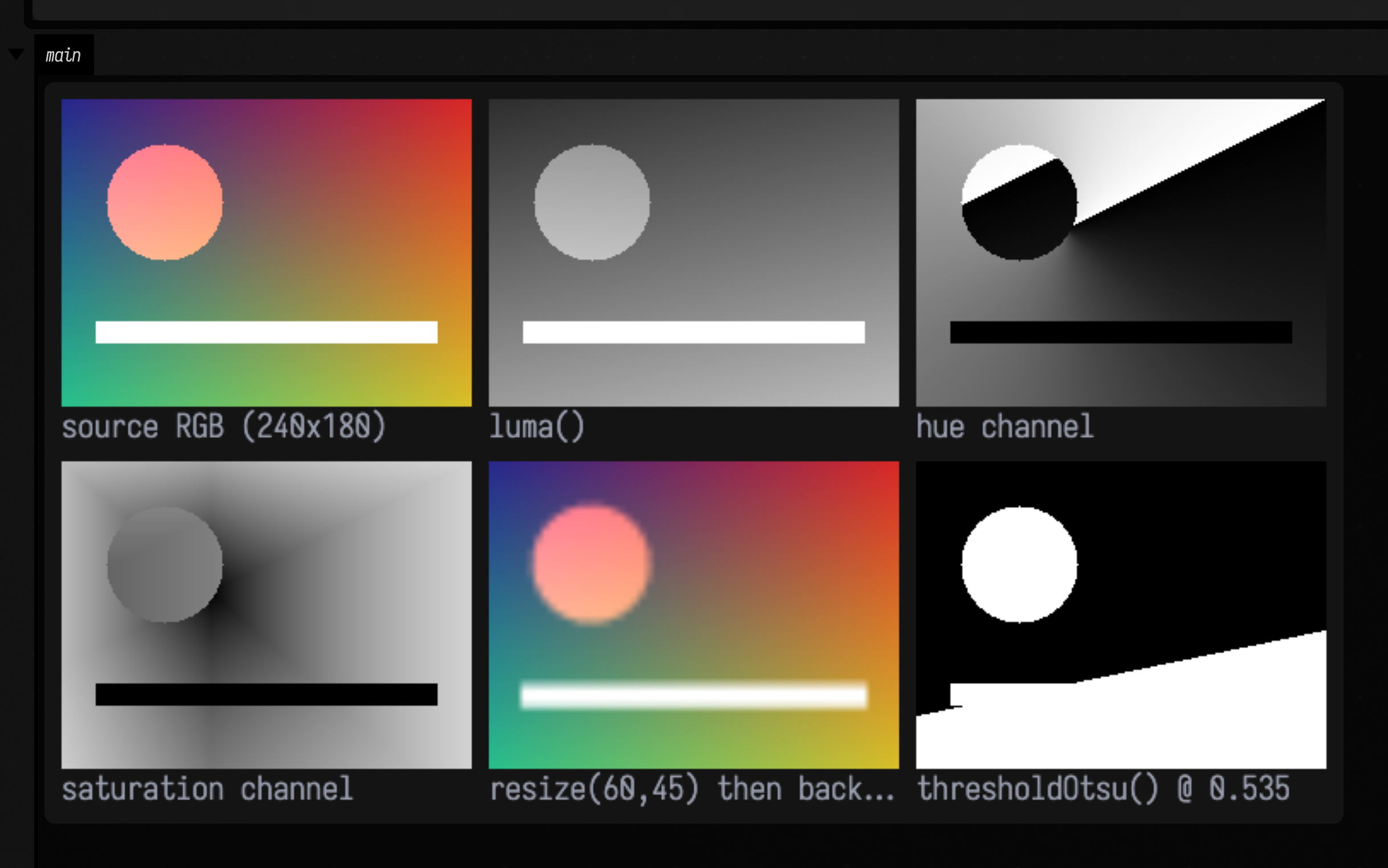
showImgGrid(...) is the fastest way to see a whole pipeline: it lays captioned panels out side by
side, maps every panel through one shared display range, and pushes one PNG to the box output through
Img.toPngBytes() → PngEncoder → display(...). Ordinary images use 0..1; out-of-range panels
choose one common automatic range, or you can pass displayRange = -1f..1f (for example). No AWT is
involved, so it works anywhere.
Choosing a filter
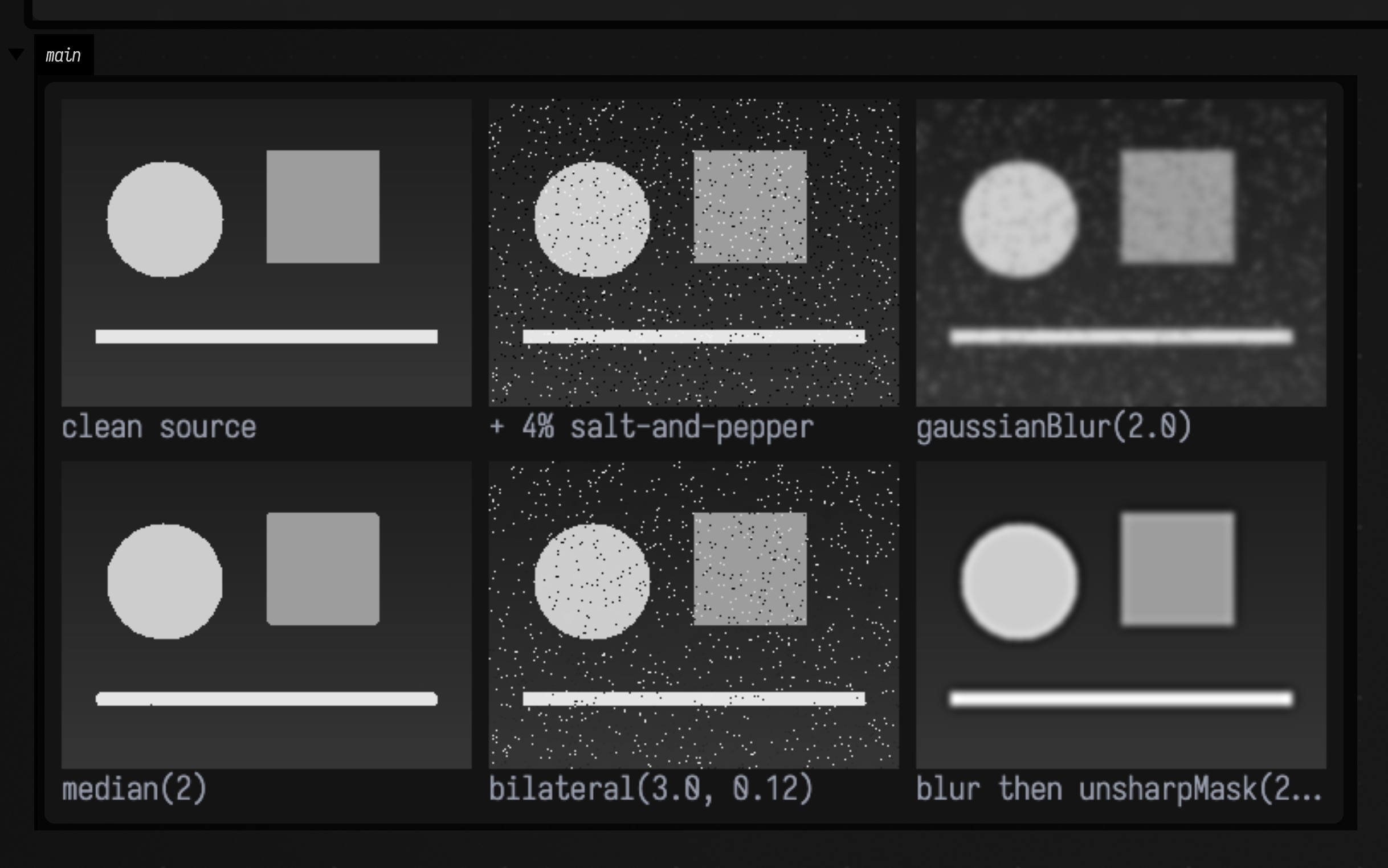
This box runs four smoothers over the same noisy image and prints each one's residual against the clean source. On impulse noise the median is two orders of magnitude better than the Gaussian. The bilateral filter, which is excellent at preserving edges, is bad at impulses: a salt pixel is far away in range and so keeps its own weight.
:::static
// A clean synthetic source, and the same source with 4% salt-and-pepper corruption.
val clean =
    Img.generate(240, 180) { x, y ->
        var v = 0.12f + 0.10f * (y / 180f)
        if (hypot(x - 60.0, y - 70.0) <= 34.0) v = 0.85f
        if (x in 120..185 && y in 30..95) v = 0.65f
        if (y in 135..142 && x in 20..219) v = 0.95f
        v
    }
val rng = kotlin.random.Random(11)
val noisy = clean.copy()
repeat((noisy.pixelCount * 0.04).toInt()) {
    noisy.data[rng.nextInt(noisy.pixelCount)] = if (rng.nextBoolean()) 0f else 1f
}

val gauss = noisy.gaussianBlur(2.0) // separable, normalised: preserves the image mean
val med = noisy.median(2) // the right tool for impulse noise
val bil = noisy.bilateral(sigmaSpace = 3.0, sigmaRange = 0.12)
val sharp = clean.gaussianBlur(2.0).unsharpMask(sigma = 2.0, amount = 1.4)

showImgGrid(
    "clean source" to clean,
    "+ 4% salt-and-pepper" to noisy,
    "gaussianBlur(2.0)" to gauss,
    "median(2)" to med,
    "bilateral(3.0, 0.12)" to bil,
    "blur then unsharpMask(2.0, 1.4)" to sharp,
    columns = 3,
    cellSide = 260,
)
println(
    "residual vs clean — gaussian ${gauss.meanAbsDiff(clean).f4}, " +
        "median ${med.meanAbsDiff(clean).f4}, " +
        "bilateral ${bil.meanAbsDiff(clean).f4}",
)
boxBlur(radius) is also there, computed with running sums so its cost is independent of the
radius, and boxBlurApproxGaussian(sigma) chains three of them when sigma is large and you care
more about speed than about the exact kernel shape.
Gradients, edges, and the FLines they become
sobel() returns a Gradient: dx, dy, and derived magnitude(), orientation() and a
hue-encoded toColorImg(). canny() runs the four classic stages (smooth, gradient, non-maximum
suppression, hysteresis) and returns a thin binary mask. toContourFLines(...) traces that mask and
hands back drawable FLines, simplified with Ramer–Douglas–Peucker so a staircase pixel boundary
becomes a handful of straight runs.
:::static
val src =
    Img.generate(240, 180) { x, y ->
        var v = 0.12f + 0.08f * (y / 180f)
        if (hypot(x - 62.0, y - 70.0) <= 34.0) v = 0.85f
        if (x in 120..185 && y in 30..95) v = 0.68f
        val tx = x - 210.0
        val ty = y - 40.0
        if (ty in 0.0..60.0 && kotlin.math.abs(tx) <= ty * 0.5) v = 0.95f
        v
    }

// Sobel here is scaled to true units-per-pixel: a unit step edge integrates to 1.
val grad = src.sobel()
val edges = src.canny(low = 0.05, high = 0.11, sigma = 1.2)
val auto = src.cannyAuto() // thresholds derived from this image's own gradients

// Edges are geometry, and geometry in Field is an FLine.
val flines = edges.toContourFLines(minPerimeter = 12, simplifyTolerance = 1.2)

showImgGrid(
    "source" to src,
    "sobel().dx (signed, coolwarm)" to grad.dx.colormapDiverging("coolwarm"),
    "sobel().dy (signed, coolwarm)" to grad.dy.colormapDiverging("coolwarm"),
    "magnitude (inferno)" to grad.magnitude().normalized().colormap("inferno"),
    "orientation as hue x magnitude" to grad.toColorImg(),
    "canny(0.05, 0.11)" to edges,
    columns = 3,
    cellSide = 260,
)
println(
    "|grad| max ${grad.magnitude().max().f3}; " +
        "canny ${edges.data.count { it > 0.5f }} px, cannyAuto ${auto.data.count { it > 0.5f }} px; " +
        "${flines.size} FLines, ${flines.sumOf { it.nodes.size }} nodes total",
)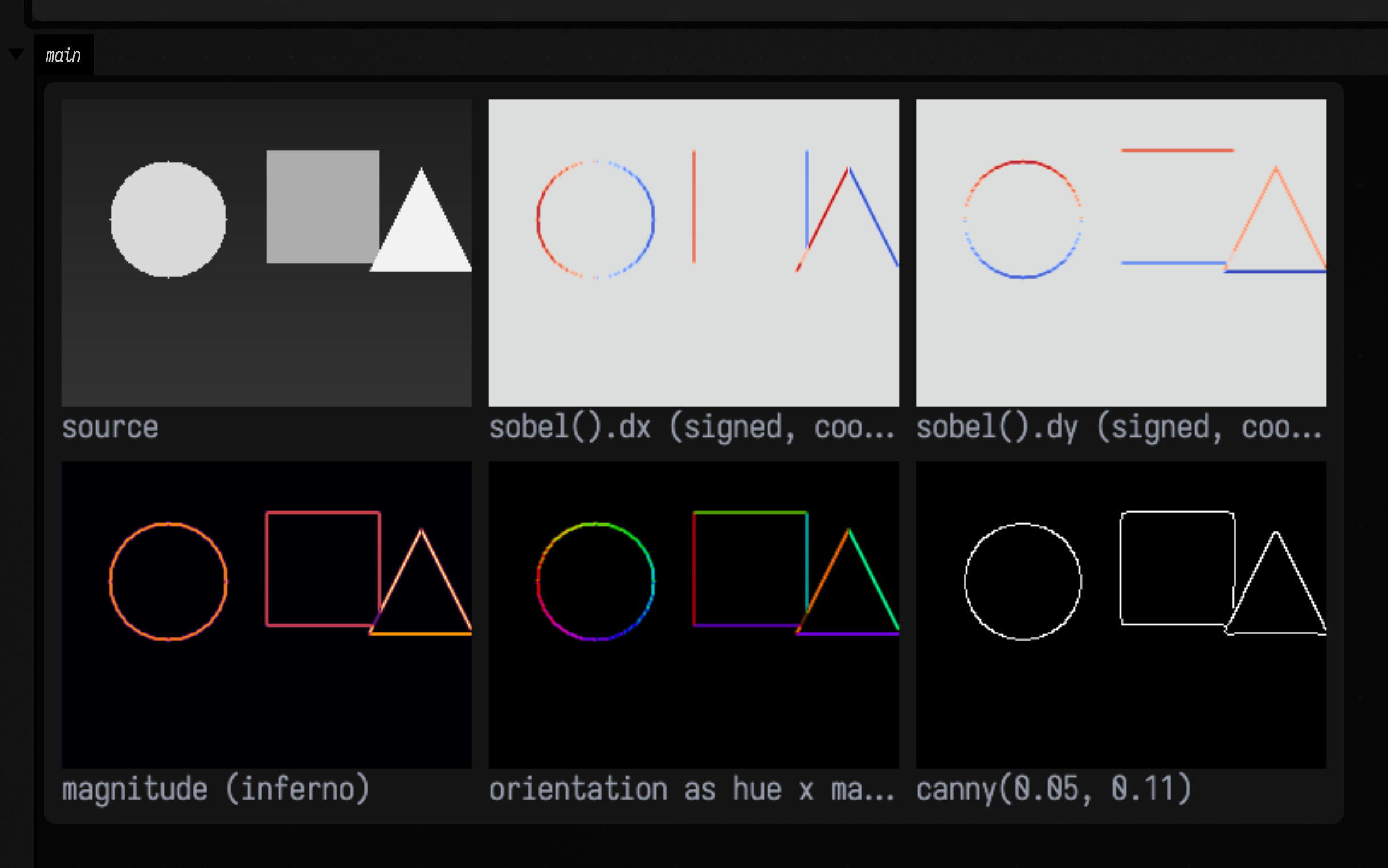
dx fires on vertical edges and dy on horizontal ones; the orientation panel wheels its hue right
around the disc, because that is what the gradient direction does.
Canny on low-contrast images
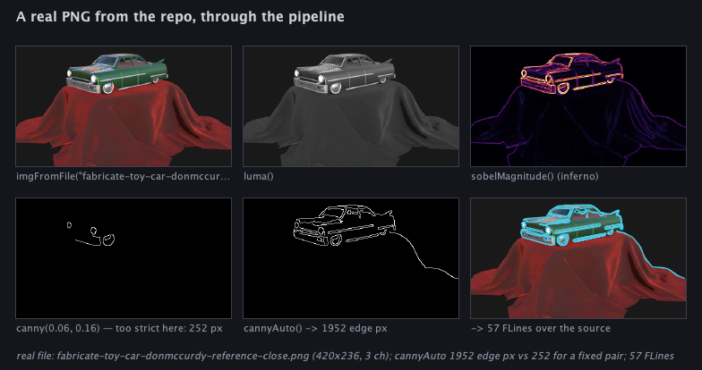
A (low, high) pair tuned on a bright synthetic card finds almost nothing in a dark, softly-lit
photograph. The thresholds are in gradient-magnitude units, and a dark image does not reach them.
cannyAuto(...) derives them from the image's own distribution: it takes a percentile of the
non-maximum-suppressed magnitudes as the strong seed threshold and Canny's own recommended ratio for
the weak one.
The figure below is a real repo PNG run through the whole pipeline. The fixed pair finds 252 edge
pixels, barely the car at all. cannyAuto() finds 1952, and traces the whole silhouette; the last
panel is those edges as 57 FLines drawn back over the source.
Corners
Three detectors, all on a square whose corners are at exactly known coordinates, so each detector's answer can be measured against the truth.
harrisResponse()— \( \det(M) - k\,\operatorname{trace}(M)^2 \) over the structure tensor. Large and positive at a corner, negative along an edge, near zero on flat ground; the diverging colour map in the figure is showing exactly that sign structure.shiTomasiResponse()— the smaller eigenvalue of the same tensor. No magick, and directly interpretable: it is the weakest intensity variation over any direction, so a large value means the point is localisable in both axes. A straight edge scores ~0, which is the aperture problem stated numerically. This is the response an optical-flow tracker wants, andgoodFeaturesToTrack(...)is its friendlier name.fastCorners()— no gradients and no eigenvalues, just a wrap-around run-length test on a 16-pixel circle. Much faster, and it scores each corner by the largest threshold at which it would still qualify.
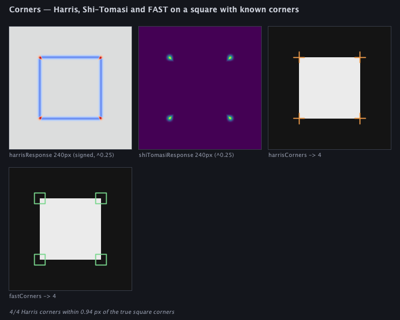
The two response maps are drawn from a 240 px copy of the square, shown 1:1, and raised to the 0.25 power so the weak values show.
Run headless, Harris and Shi–Tomasi each return exactly four corners, and the worst of the four sits
0.94 px from the true corner of the square (sub-pixel refinement is on by default, via a
three-tap parabola fit in x and y). cornersToFLines(...) turns them into drawable crosses or boxes.
Hough lines
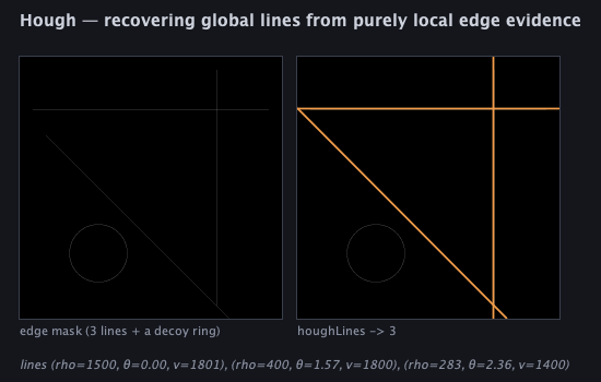
Every edge pixel votes for every line through it; a real line becomes a bright peak in (rho, theta)
accumulator space, with no grouping step in between.
The figure has three planted lines and a decoy ring. All three lines come back at their exact polar
coordinates: (rho=1500, θ=0.00), (rho=400, θ=1.57), (rho=283, θ=2.36). The ring is not
fitted.
HoughLine.clipTo(w, h) clips the infinite line to the image rectangle, and linesToFLines(...)
gives you the visible segments as FLines. houghCircles(...) is there too, for a known radius
range.
Morphology, blobs and distance
erode / dilate / open / close with square, disc or cross structuring elements;
connectedComponents(...) for labels plus per-blob area, bounding box, centroid and fill ratio;
distanceTransform() for the exact Euclidean distance to the nearest background pixel (the
Felzenszwalb–Huttenlocher two-pass algorithm, not a chamfer approximation).
:::static
// Three disjoint discs of known radius, then noise on top of them.
val discs = [Triple(55.0, 60.0, 28.0), Triple(150.0, 55.0, 20.0), Triple(110.0, 135.0, 14.0)]
val clean =
    Img.generate(220, 180) { x, y ->
        if (discs.any { (cx, cy, r) -> hypot(x - cx, y - cy) <= r }) 0.85f else 0.15f
    }
val rng = kotlin.random.Random(3)
val noisy = clean.copy()
repeat((noisy.pixelCount * 0.03).toInt()) {
    noisy.data[rng.nextInt(noisy.pixelCount)] = if (rng.nextBoolean()) 0f else 1f
}

val mask = noisy.thresholdOtsu()
val cleaned = mask.open(2, StructuringElement.DISC).close(2, StructuringElement.DISC)
val cc = cleaned.connectedComponents(8)
val dt = cleaned.distanceTransform()

showImgGrid(
    "noisy source" to noisy,
    "thresholdOtsu()" to mask,
    "open(2,DISC).close(2,DISC)" to cleaned,
    "erode(4)" to cleaned.erode(4, StructuringElement.DISC),
    "dilate(4)" to cleaned.dilate(4, StructuringElement.DISC),
    "distanceTransform (magma)" to dt.normalized().colormap("magma"),
    columns = 3,
    cellSide = 250,
)
println("${cc.count} components after cleaning (planted ${discs.size} discs):")
cc.components
    .sortedByDescending { it.area }
    .forEach {
        println(
            "  area=${it.area} centroid=(${it.centroidX.f1}, ${it.centroidY.f1}) " +
                "bbox=${it.boundingWidth}x${it.boundingHeight} fill=${it.fillRatio.f2}",
        )
    }
println("distance-transform peak ${dt.max().f1} (largest planted radius ${discs.maxOf { it.third }})")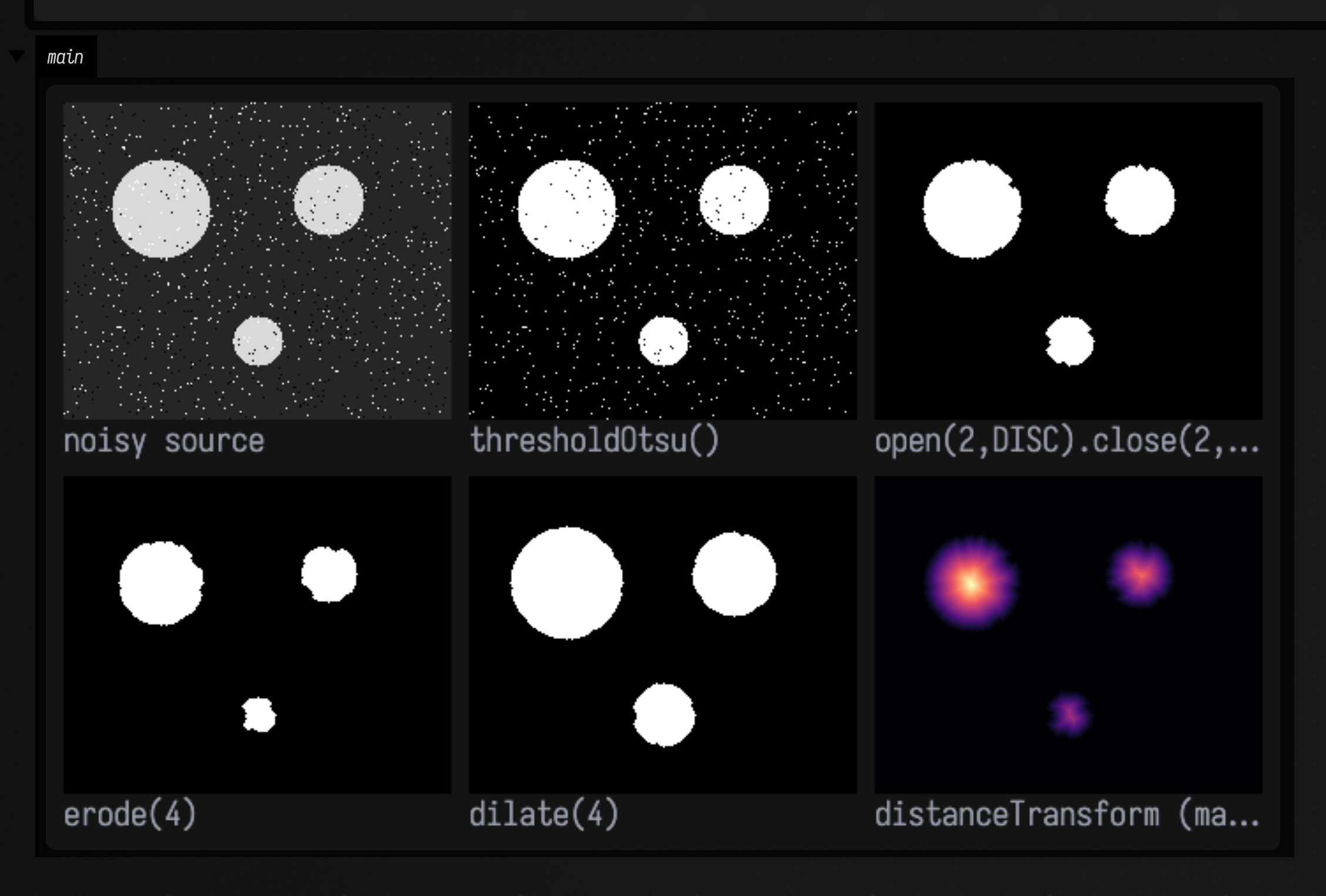
Three discs in, three components out, with areas of 2419, 1226 and 584 against the analytic
\( \pi r^2 \) of 2463, 1257 and 616 (the shortfall is the open(2) erosion), and centroids at (54.8, 60.1),
(150.1, 55.0) and (110.2, 134.9) against planted centres of (55, 60), (150, 55) and (110, 135).
For sub-pixel-smooth contours rather than a pixel-staircase boundary, isoContourFLines(iso) adapts
the image to the ScalarField2D that Field's existing marching-squares extractor
(contours) already marches, so a distance transform or a blurred response
becomes a smooth curve with no glue code.
Multiscale
gaussianPyramid(levels) halves each octave (blurring first, so it does not alias);
laplacianPyramid(levels) splits the image into band-pass detail plus a coarse residual, and
reconstruct() inverts it. The round-trip is exact to within float precision, at a maximum
absolute error of 5.96e-08 on the figure below. That is small enough to build multiband
blending and detail transfer on, rather than only to look at.
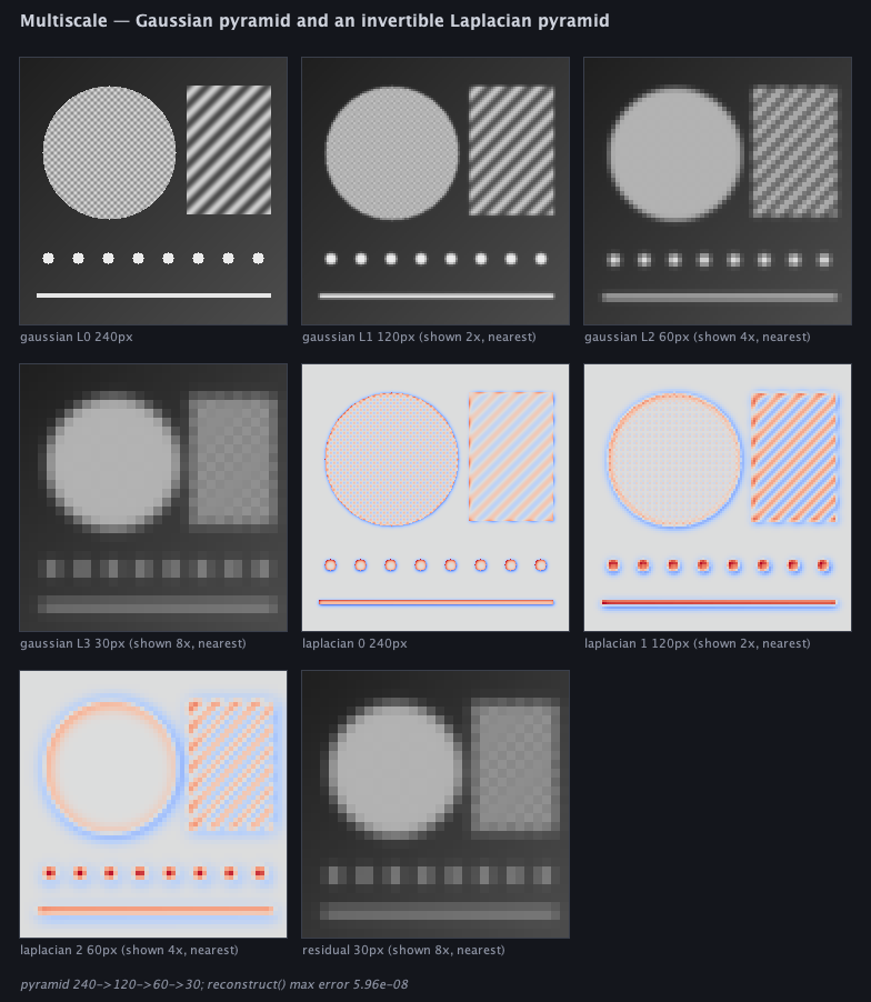
(Levels below the base are magnified by integer pixel replication for display; each caption states the real size and the zoom factor.)
Geometry — affine and projective warps
Affine2D uses the same six-number layout as java.awt.geom.AffineTransform and SVG's
matrix(a, b, c, d, e, f). Homography is the 3×3 projective version. warpAffine and
warpPerspective map source → destination and invert internally, doing the correct backwards
resample, so there are no holes.
findHomography(src, dst) is the Direct Linear Transform: exact through four correspondences,
least-squares through more. The points are Hartley-normalised first; without that, the conditioning
on pixel-scale coordinates is bad enough to visibly distort the fit.
warpQuadToRect(quad, w, h) wraps it up as the "flatten the photographed page" operation.
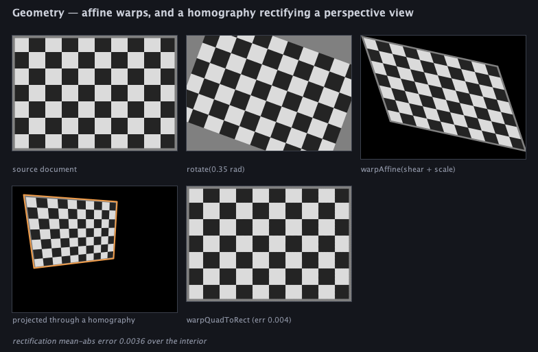
The rectified checkerboard matches the original to a mean absolute error of 0.0036 over the interior.
Motion
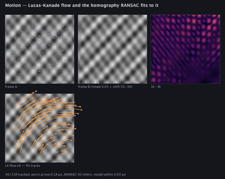
opticalFlowLK(a, b, points) is pyramidal Lucas–Kanade. Seed it with goodFeaturesToTrack(...),
which selects exactly the points where the 2×2 tracking system is well conditioned, and it returns
a FlowField of FlowVectors, each of which reports whether it converged. A track is marked
ok = false when the system is ill-conditioned (a smooth region, or a straight edge) or the point
leaves the frame.
The pyramid is there for large motions. Solve at the coarsest octave, where the displacement is small enough for the linearisation to hold, then propagate the estimate down. A 9-pixel shift that a single level cannot recover comes back to within half a pixel with four.
:::static
// Two frames related by a transform we choose, so the answer is known in advance.
val a =
    Img.generate(200, 200) { x, y ->
        (0.5 + 0.24 * kotlin.math.sin(x * 0.21) * kotlin.math.cos(y * 0.17) + 0.16 * kotlin.math.sin((x + y) * 0.11))
            .toFloat()
            .coerceIn(0f, 1f)
    }
val planted = Affine2D.rotationAbout(0.05, 100.0, 100.0).compose(Affine2D.translation(5.0, -3.0))
val b = a.warpAffine(planted, border = Border.CLAMP)

// Seed only where the 2x2 tracking system is well conditioned.
val seeds =
    a.goodFeaturesToTrack(maxCount = 200, minDistance = 9)
        .filter { it.x in 24.0..176.0 && it.y in 24.0..176.0 }
        .map { it.toVec2() }
val flow = opticalFlowLK(a, b, seeds, windowRadius = 8, levels = 3)
val fit = findHomographyRansac(
    flow.sourcePoints(),
    flow.targetPoints(),
    threshold = 1.5,
    iterations = 1200,
    seed = 3L,
)

// How far is the recovered model from the one we planted, in pixels, on a probe grid?
var worst = 0.0
for (gx in 40..160 step 40) for (gy in 40..160 step 40) {
    val (fx, fy) = fit.homography.apply(gx.toDouble(), gy.toDouble())
    val (tx, ty) = planted.apply(gx.toDouble(), gy.toDouble())
    worst = maxOf(worst, hypot(fx - tx, fy - ty))
}

showImgGrid(
    "frame A" to a,
    "frame B (rot 0.05 rad + shift 5,-3)" to b,
    "|A - B| (inferno)" to frameDifference(a, b).normalized().colormap("inferno"),
    "B warped back by the fitted model" to b.warpPerspective(fit.homography.inverse(), border = Border.CLAMP),
    columns = 2,
    cellSide = 280,
)
val (mdx, mdy) = flow.medianDisplacement()
println(
    "${flow.tracked().size}/${seeds.size} tracked; median displacement " +
        "(${mdx.f2}, ${mdy.f2}) px",
)
println("RANSAC ${fit.inlierCount} inliers of ${flow.tracked().size} after ${fit.iterations} iterations")
println("recovered model agrees with the planted transform to ${worst.f3} px over the probe grid")
println(fit.homography.toString())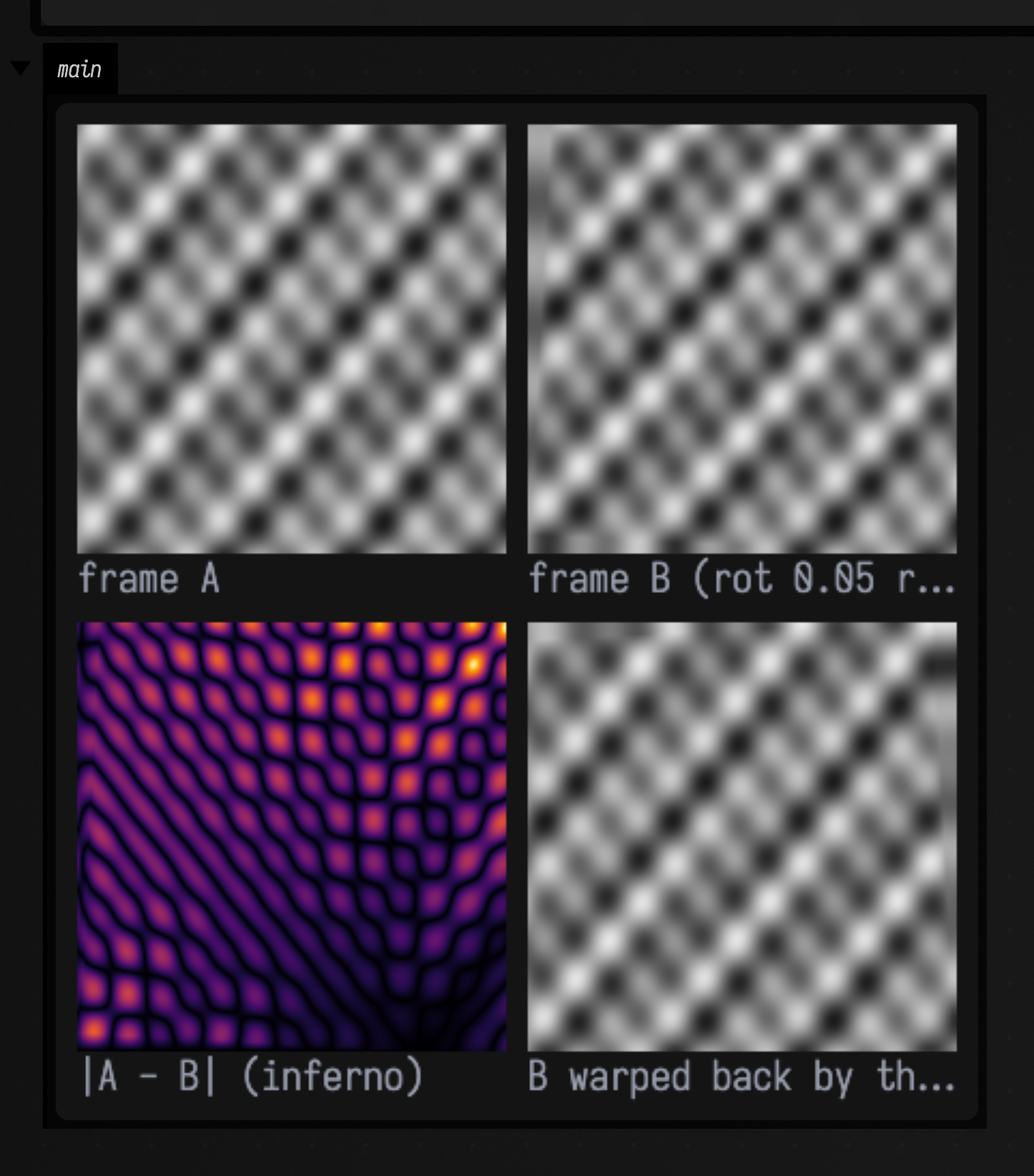
With findHomographyRansac(...) half the correspondences can be garbage and the answer is still
right, because a wrong model has no reason to be consistently wrong across many points. It samples
four correspondences at a time, scores the consensus, keeps the
best, and refits least-squares on the inliers. The seed is explicit, so a docs capture or a test
gets the same answer every time.
opticalFlowBlockMatch(...) is the brute-force alternative for displacements large enough to break
Lucas–Kanade's linearisation, and frameDifference(...) / updateBackground(...) are the crude,
reliable motion cues; pair them with open(...) to drop sensor noise and connectedComponents(...)
to count what moved.
FlowField.toFLines(scale, ...) draws the whole field as arrows, shaft plus arrowhead, so direction
is visible and not just magnitude:
Colour
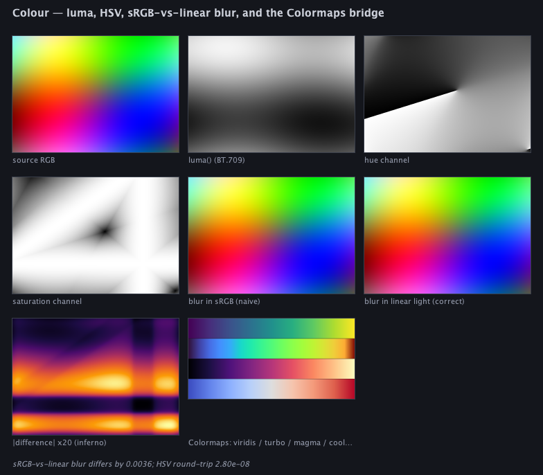
luma(), rgbToHsv() / hsvToRgb(), and toLinear() / toSrgb(). Blurring, downsampling and
averaging are only correct in linear light, so img.toLinear().gaussianBlur(4.0).toSrgb() is
measurably different from blurring the encoded values. The panel below shows both, and the
amplified difference between them.
colormap(name, lo, hi) runs a 1-channel image through any of the Colormaps ramps (viridis,
magma, inferno, plasma, turbo, coolwarm, grayscale); colormapDiverging(name) picks a
symmetric range around zero, the right default for anything signed.
Trying it yourself
The imaging_cv_examples starting point builds the
examples on this page as live boxes. Change a sigma, a threshold or the planted motion, re-run the
box, and watch the picture update.
Agents: where the figures come from
The images under the code fences are those boxes' own output, captured by the docs build. The
figures without a fence come from the imaging.gallery FIELD_TEST
(python3 tools/run_field_tests.py --id imaging.gallery), which builds each one from real Img
pipelines and fails if Canny stops being thinner than a raw threshold, the corner marks drift
off the square's corners, Hough stops recovering the planted lines, the Laplacian pyramid stops
round-tripping, or a flow arrow disagrees with the planted motion.
Speed, against OpenCV
These filters are pure Kotlin with no native dependency. The repository carries a benchmark that
puts them beside OpenCV in the same JVM, on the same pixels: tools/imaging-bench, run with
./gradlew :tools:imaging-bench:jmhThe table below compares the two in milliseconds per call.
How the kernels are written
Underneath is a small layer of vectorized span kernels (Java Vector API, imaging_simd.kt).
Three operations are fast mostly because they do less work: pyrDown filters only the rows and
columns that survive the decimation, boxBlur accumulates a row at a time instead of a column,
and bilateral reads a table instead of calling Math.exp per tap.
dev_docs/IMAGING_VECTOR_KERNELS.md describes the layer and has the checklist for adding an
operator.
| operation | before (scalar) | now | OpenCV 4.9, 1 thread | now vs OpenCV |
|---|---|---|---|---|
| Gaussian blur, sigma 2, gray | 91.59 ± 2.61 | 7.09 ± 0.07 | 7.13 ± 0.39 | 0.99x |
| Gaussian blur, sigma 2, RGB | 263 ± 8.68 | 19.61 ± 0.15 | 21.81 ± 0.48 | 0.90x |
| Sobel | 52.94 ± 0.13 | 4.49 ± 0.04 | 2.09 ± 0.03 | 2.14x |
| Scharr | — | 4.49 ± 0.04 | 2.21 ± 0.03 | 2.03x |
| Laplacian | — | 2.68 ± 0.02 | 1.61 ± 0.08 | 1.66x |
| Dense 11x11 convolution | — | 26.19 ± 0.21 | 27.22 ± 0.91 | 0.96x |
| Luma (RGB to gray) | — | 1.96 ± 0.01 | 1.14 ± 0.01 | 1.72x |
| Box blur, radius 2 | — | 2.60 ± 0.03 | 1.89 ± 0.10 | 1.38x |
| Median, radius 2 | — | 425 ± 5.30 | 120 ± 7.82 | 3.53x |
| Resize to half | — | 3.65 ± 0.06 | 0.73 ± 0.01 | 4.99x |
| Bilateral | — | 749 ± 95.18 | 628 ± 4.25 | 1.19x |
| pyrDown | — | 2.07 ± 0.02 | 0.50 ± 0.02 | 4.12x |
Bold means we are faster. A dash in the "before" column means that operation has no preserved scalar original to compare against, not that its speedup is unknown.
Gaussian blur, box blur and the Laplacian run the same operation with the same parameters on both
sides, and the benchmark fails if their outputs stop agreeing. The rest are matched in work but not
in definition, so their ratios compare slightly different operations: our luma is BT.709 where
cvtColor is BT.601; our Sobel and Scharr are scaled to true units-per-pixel, so ours is OpenCV's
divided by a constant; our pyrDown takes a configurable sigma where OpenCV's is a fixed 5-tap
kernel; and median/bilateral have matched parameters but different internal algorithms. Our API
also returns a fresh Img each call, so part of our cost is an allocation OpenCV is not paying.
Gaussian blur, dense convolution and the RGB blur are at or slightly past OpenCV; box blur, the
Laplacian, Scharr, Sobel, luma and bilateral are all inside about 2x, close enough that the
pure-Kotlin path is the reasonable default. bilateral's interval is wide, so read its row as
"about 1.2x". Three rows are meaningfully behind, and you should know which before choosing:
medianis an algorithmic gap: it sorts 25 floats per pixel where OpenCV uses a sorting network.resizeto half has data-dependent inner loops that do not vectorize.pyrDownis doing more arithmetic, not doing it worse: ours appliesgaussianKernel1D(sigma), 9 taps at the default, where OpenCV'spyrDownis a fixed 5-tap[1,4,6,4,1]/16. That is close to twice the work, in exchange for a better filter and a sigma that is yours to choose.
The benchmark's conditions, the agreement tolerances, and what the absolute milliseconds depend on
are in dev_docs/IMAGING_MEASUREMENTS.md.
Reference
Value type
Load, construct and save floating-point images.
| Entry point | Behavior |
|---|---|
Img |
A CPU raster image: width * height * channels floats, interleaved, row-major, origin top-left (the image-processing convention, matching BufferedImage and PNG). API. |
Border |
How a filter resolves coordinates that fall outside the image. API. |
fun imgFromFile(path: String, channels: Int? = null): Img |
Loads an image from a file path, straight through ImageIO — the path is used verbatim and does not go through FileManager, so a workspace-relative spec will not resolve here. API. |
fun imgFromBytes(bytes: ByteArray, channels: Int? = null): Img |
Decode an image from in-memory encoded bytes (PNG/JPEG/… — whatever ImageIO handles). API. |
fun floatsToImg(values: FloatArray, width: Int, height: Int): Img |
Wrap a plain FloatArray of scalars as a 1-channel image — the bridge from the rest of the stdlib (a heightfield, a spectrogram frame stack, a DoubleArray reduction) into imaging. API. |
fun Img.toBufferedImage(): BufferedImage |
Convert to a BufferedImage for AWT drawing / ImageIO. Samples are clamped to 0..1 and quantised to 8 bits at this point (and only at this point). A 1-channel image becomes gray RGB. API. |
fun Img.toPngBytes(): ByteArray |
Encode straight to PNG bytes with no AWT (via PngEncoder) — the path a box uses to put a picture in its own output, and the path Img.toHTML uses for its thumbnail. API. |
fun Img.savePng(path: String): File |
Write this image to path as a PNG (creating parent directories). Returns the file. API. |
Sampling / shape
Change the image extent or sample positions. Use nearest sampling for discrete labels and bilinear sampling for interpolated image values.
| Entry point | Behavior |
|---|---|
fun Img.sampleNearest(x: Double, y: Double, c: Int = 0, border: Border = Border.CLAMP): Float |
Nearest-neighbour sample at continuous coordinates. API. |
fun Img.sampleBilinear(x: Double, y: Double, c: Int = 0, border: Border = Border.CLAMP): Float |
Bilinear sample at continuous coordinates — pixel centres sit at integer coordinates, so sampleBilinear(3.0, 4.0) == at(3, 4) exactly. API. |
fun Img.crop(x: Int, y: Int, w: Int, h: Int): Img |
Rectangular sub-image. Coordinates are clamped into range; the result is at least 1x1. API. |
fun Img.pad(pad: Int, border: Border = Border.CLAMP): Img |
Grow the image by pad pixels on every side, filling from border. API. |
fun Img.resize(newWidth: Int, newHeight: Int, areaAverage: Boolean = true): Img |
Resize to newWidth x newHeight. API. |
fun Img.scaleBy(factor: Double, areaAverage: Boolean = true): Img |
Resize by a scale factor (both axes). See resize. API. |
fun Img.flipX(): Img |
Mirror left-right. API. |
fun Img.flipY(): Img |
Mirror top-bottom. API. |
fun Img.rotate90(): Img |
Rotate 90 degrees clockwise (width and height swap). API. |
fun Img.transpose(): Img |
Transpose (x and y swap). API. |
Channels / colour
Select channels or change colour representations.
| Entry point | Behavior |
|---|---|
fun Img.channel(c: Int): Img |
Extract channel c as a 1-channel image. API. |
fun Img.split(): List<Img> |
Split into one 1-channel image per channel. API. |
fun mergeChannels(vararg parts: Img): Img |
Merge 1-channel images into a multi-channel image. All inputs must share a shape and the count must be 1, 3 or 4. API. |
fun Img.luma(): Img |
Perceptual grayscale (BT.709 luma) as a 1-channel image. A 1-channel input is returned as a copy; an RGBA input ignores alpha. API. |
fun Img.toRGB(): Img |
Replicate a 1-channel image into 3 channels (the inverse direction of luma). API. |
fun Img.toRGBA(alpha: Float = 1f): Img |
Add an opaque (or alpha-valued) alpha channel. API. |
fun Img.toLinear(): Img |
Decode sRGB-encoded samples to linear light. Blurring, downsampling and averaging are only correct in linear light; img.toLinear().gaussianBlur(2.0).toSrgb() is the physically right blur, and visibly different from blurring the encoded values. API. |
fun Img.toSrgb(): Img |
Encode linear-light samples back to sRGB. Inverse of toLinear. API. |
fun Img.rgbToHsv(): Img |
RGB → HSV, in place of the channels: h in 0..1 (hue angle / 360), s in 0..1, v in 0..1. Requires a 3- or 4-channel image; alpha is dropped. API. |
fun Img.hsvToRgb(): Img |
HSV → RGB, the inverse of rgbToHsv. API. |
Statistics
Measure or remap intensity distributions.
| Entry point | Behavior |
|---|---|
fun normalized(): Kernel1D |
A copy scaled so the taps sum to 1. Throws for a zero-sum (derivative) kernel. API. |
fun Img.normalizedPercentile(pLow: Double = 0.01, pHigh: Double = 0.99): Img |
Robust normalisation: map the pLow/pHigh percentiles of the sample distribution to 0..1 and clamp. Far more useful than normalized on noisy gradient/response images, where one hot pixel otherwise squashes everything else to black. API. |
fun Img.histogram(bins: Int = 256, lo: Float = 0f, hi: Float = 1f): IntArray |
Histogram of a 1-channel image over [lo, hi] with bins equal-width buckets. Values outside the range land in the first/last bucket. API. |
fun Img.equalize(bins: Int = 256): Img |
Histogram equalisation of a 1-channel image: remap intensities through the cumulative histogram so the output distribution is (approximately) flat. Classic contrast enhancement. API. |
fun Img.otsuThreshold(bins: Int = 256): Float |
Otsu's method: the intensity threshold in [lo, hi] that maximises between-class variance — i.e. the best two-way split of a bimodal histogram, computed rather than guessed. API. |
fun Img.threshold(threshold: Float): Img |
Binarise: samples > threshold become 1, everything else 0. Result is 1-channel. API. |
fun Img.thresholdOtsu(bins: Int = 256): Img |
Binarise at the otsuThreshold. API. |
fun Img.thresholdAdaptive(radius: Int = 8, bias: Float = 0.02f): Img |
Adaptive (local-mean) threshold: each pixel is compared to the mean of a (2*radius+1) square neighbourhood, minus bias. Handles uneven illumination that defeats a global threshold. API. |
fun Img.meanAbsDiff(other: Img): Double |
Mean absolute difference per sample against other — a blunt but unbiased similarity measure. API. |
fun Img.psnr(other: Img): Double |
Peak signal-to-noise ratio in dB against other, assuming a 0..1 signal range. API. |
Filters
Smooth, sharpen or apply a custom kernel.
| Entry point | Behavior |
|---|---|
Kernel1D |
A 1-D convolution kernel: taps centred on the middle element (so the length is normally odd). API. |
Kernel2D |
A dense 2-D convolution kernel, width x height, centred (odd dimensions expected). API. |
fun Img.convolveSeparable(kx: Kernel1D, ky: Kernel1D? = kx, border: Border = Border.CLAMP): Img |
Separable convolution: kx along x then ky along y (or kx both ways if ky is null). O(kx + ky) per pixel per channel. API. |
fun Img.convolve2D(k: Kernel2D, border: Border = Border.CLAMP): Img |
Dense 2-D convolution with k. True convolution (the kernel is flipped); pass an already-flipped kernel or a symmetric one if you want correlation. O(kw * kh) per pixel per channel — this is the general fallback, and the reference the separable path is tested against. API. |
fun Img.correlate2D(k: Kernel2D, border: Border = Border.CLAMP): Img |
Cross-correlation with k (kernel not flipped). This is what most "apply this stencil" intuitions actually mean; identical to convolve2D for symmetric kernels. API. |
fun Img.gaussianBlur(sigma: Double, truncate: Double = 4.0, border: Border = Border.CLAMP): Img |
Gaussian blur with standard deviation sigma, run as two separable 1-D passes. API. |
fun Img.boxBlur(radius: Int, border: Border = Border.CLAMP): Img |
Box (mean) blur over a (2*radius+1)² window, computed with running sums so the cost is independent of radius. API. |
fun Img.boxBlurApproxGaussian(sigma: Double, border: Border = Border.CLAMP): Img |
Three successive boxBlur passes, which by the central limit theorem approximate a Gaussian of standard deviation sigma — O(1) per pixel at any sigma. Use when sigma is large and you care more about speed than about the exact kernel shape. API. |
fun Img.median(radius: Int = 1, border: Border = Border.CLAMP): Img |
Median filter over a (2*radius+1)² window — the standard salt-and-pepper de-noiser, and unlike a mean it does not smear edges. API. |
fun Img.bilateral(sigmaSpace: Double = 3.0, sigmaRange: Double = 0.1, border: Border = Border.CLAMP): Img |
Bilateral filter: a Gaussian blur whose weights are additionally attenuated by intensity distance, so it smooths flat regions while leaving edges sharp. API. |
fun Img.unsharpMask(sigma: Double = 1.5, amount: Double = 1.0, threshold: Float = 0f): Img |
Unsharp mask: image + amount * (image - gaussianBlur(image, sigma)). The oldest sharpening trick there is; threshold suppresses amplification of low-contrast noise. API. |
Gradients
Measure spatial changes in intensity.
| Entry point | Behavior |
|---|---|
Gradient |
A gradient field: per-pixel partial derivatives of a scalar image. API. |
fun Img.sobel(border: Border = Border.CLAMP): Gradient |
Sobel gradients. The 3x3 Sobel operator factors into a [-1, 0, 1] derivative across the gradient axis and a [1, 2, 1]/4 smoothing along it, so both components run separably. API. |
fun Img.sobelMagnitude(border: Border = Border.CLAMP): Img |
Shorthand for sobel().magnitude(). API. |
fun Img.scharr(border: Border = Border.CLAMP): Gradient |
Scharr gradients — same structure as sobel but with the [3, 10, 3]/16 smoothing factor, which has markedly better rotational symmetry (the direction estimate is more accurate on diagonal edges). API. |
fun Img.gaussianGradient(sigma: Double, truncate: Double = 4.0, border: Border = Border.CLAMP): Gradient |
Gradients of a Gaussian-smoothed image at scale sigma, computed as the analytic derivative of the Gaussian (not a blur followed by a difference), so the scale is exact. API. |
fun Img.laplacian(eightNeighbour: Boolean = false, border: Border = Border.CLAMP): Img |
Discrete Laplacian (second derivative). eightNeighbour picks LAPLACIAN_8 over LAPLACIAN_4. API. |
fun Img.laplacianOfGaussian(sigma: Double = 1.5, border: Border = Border.CLAMP): Img |
Laplacian of Gaussian at scale sigma — computed as the difference of the image and its blur's Laplacian, i.e. laplacian(gaussianBlur(img, sigma)). Zero crossings are edges at that scale. API. |
fun Img.differenceOfGaussians(sigma1: Double = 1.0, sigma2: Double = 2.0, border: Border = Border.CLAMP): Img |
Difference of Gaussians, blur(sigma1) - blur(sigma2) with sigma1 < sigma2 — the cheap band-pass approximation to laplacianOfGaussian and the basis of blob detection. API. |
Multiscale
Build coarse-to-fine image representations.
| Entry point | Behavior |
|---|---|
fun Img.pyrDown(sigma: Double = 1.0): Img |
One-octave downsample: blur by sigma then take every other pixel. The blur is what keeps this from aliasing — a bare decimation of a fine texture produces moiré, not a small picture. API. |
fun Img.pyrUp(targetWidth: Int = width * 2, targetHeight: Int = height * 2, sigma: Double = 1.0): Img |
One-octave upsample to exactly targetWidth x targetHeight (default 2x), bilinear then smoothed by sigma to suppress the interpolation grid. The approximate inverse of pyrDown. API. |
fun Img.gaussianPyramid(levels: Int = 4, sigma: Double = 1.0, minSize: Int = 8): GaussianPyramid |
Build a GaussianPyramid with at most levels octaves, stopping at minSize pixels. API. |
fun Img.laplacianPyramid(levels: Int = 4, sigma: Double = 1.0, minSize: Int = 8): LaplacianPyramid |
Build a LaplacianPyramid: at each octave, band = level - pyrUp(pyrDown(level)). The reconstruction is exact up to the upsampling filter, so it is a genuine invertible band-splitting — the basis of multiband blending, texture synthesis and detail transfer. API. |
Edges / features
Find edge pixels or repeatable corner locations. Use corner responses when you need a score image, and corner detectors when you need point coordinates.
| Entry point | Behavior |
|---|---|
fun Img.canny(low: Double = 0.08, high: Double = 0.20, sigma: Double = 1.0): Img |
Canny edge detection. API. |
fun Img.cannyAuto(highPercentile: Double = 0.90, lowRatio: Double = 0.4, sigma: Double = 1.0): Img |
canny with the thresholds chosen from the image instead of guessed. API. |
fun nonMaximumSuppression(magnitude: Img, gradient: Gradient): Img |
Thin a gradient-magnitude image to ridge crests: a pixel survives only if its magnitude is >= both neighbours sampled along the gradient direction (quantised to the nearest of the four 45-degree axes). Exposed because it is useful on its own, on any gradient field. API. |
fun hysteresis(thinned: Img, low: Float, high: Float): Img |
Double-threshold + connectivity: pixels above high are edges; pixels above low become edges only if 8-connected (transitively) to one. Returns a binary mask. API. |
fun Img.harrisResponse(k: Double = 0.04, sigma: Double = 1.5, gradientSigma: Double = 1.0): Img |
Harris corner response image, det(M) - k * trace(M)² over the structureTensor M. Large and positive at a corner, negative along an edge, near zero on flat ground. API. |
fun Img.shiTomasiResponse(sigma: Double = 1.5, gradientSigma: Double = 1.0): Img |
Shi–Tomasi ("good features to track") response: the smaller eigenvalue of the structure tensor. Unlike Harris it needs no magic k, and the response is directly interpretable — it is the weakest intensity variation over any direction, so a large value means the point is localisable in both axes. This is the response optical-flow trackers want. API. |
fun Img.harrisCorners(k: Double = 0.04, threshold: Double = 0.01, minDistance: Int = 5, maxCount: Int = 200, sigma: Double = 1.5): List<Corner> |
Harris corners: harrisResponse followed by peakCorners. API. |
fun Img.shiTomasiCorners(threshold: Double = 0.01, minDistance: Int = 5, maxCount: Int = 200, sigma: Double = 1.5): List<Corner> |
Shi–Tomasi corners: shiTomasiResponse followed by peakCorners. The default tracker seed. API. |
fun Img.goodFeaturesToTrack(maxCount: Int = 200, threshold: Double = 0.01, minDistance: Int = 5): List<Corner> |
Alias for shiTomasiCorners under the name the OpenCV-literate will reach for first. API. |
fun Img.fastCorners(threshold: Double = 0.08, contiguous: Int = 9, minDistance: Int = 5, maxCount: Int = 300): List<Corner> |
FAST corner detection (Rosten & Drummond): a pixel is a corner if at least contiguous of the 16 pixels on a radius-3 circle around it are all brighter than centre + t or all darker than centre - t. No gradients, no eigenvalues — just a wrap-around run-length test, which is why it is the fastest usable corner detector. API. |
fun peakCorners(response: Img, threshold: Double = 0.01, minDistance: Int = 5, maxCount: Int = 200, subPixel: Boolean = true): List<Corner> |
Peak extraction shared by the corner detectors: keep local maxima of response that clear threshold * max(response), sort by strength, and greedily drop any peak within minDistance pixels of a stronger one. API. |
fun Img.structureTensor(sigma: Double = 1.5, gradientSigma: Double = 1.0): Triple<Img, Img, Img> |
The per-pixel structure tensor (second-moment matrix) of a scalar image, Gaussian-weighted over a neighbourhood — the shared engine behind Harris, Shi–Tomasi and optical flow. API. |
Lines / blobs
Group local evidence into shapes. The morphology here runs on a mask before you label components or trace contours, not after.
| Entry point | Behavior |
|---|---|
fun houghLines(edges: Img, thetaSteps: Int = 360, rhoStep: Double = 1.0, threshold: Int = 0, maxLines: Int = 20, minSeparationTheta: Double = 0.15, minSeparationRho: Double = 12.0): List<HoughLine> |
Standard Hough line transform over a binary edge mask. API. |
fun houghCircles(edges: Img, minRadius: Int = 8, maxRadius: Int = 40, radiusStep: Int = 2, threshold: Double = 0.5, maxCircles: Int = 10, minSeparation: Double = 10.0, angleStepDeg: Double = 3.0): List<HoughCircle> |
Hough circle transform over a binary edge mask, brute force over the radius range. Each edge pixel votes for the centres of all circles of each candidate radius passing through it. API. |
fun Img.erode(radius: Int = 1, shape: StructuringElement = StructuringElement.SQUARE): Img |
Grayscale erosion: each pixel becomes the minimum over the structuring element. On a binary mask this shrinks bright regions and deletes anything thinner than the element. API. |
fun Img.dilate(radius: Int = 1, shape: StructuringElement = StructuringElement.SQUARE): Img |
Grayscale dilation: each pixel becomes the maximum over the structuring element. On a binary mask this grows bright regions and bridges gaps narrower than the element. API. |
fun Img.open(radius: Int = 1, shape: StructuringElement = StructuringElement.SQUARE): Img |
Erode then dilate — removes specks and thin protrusions, keeps the overall size of what remains. API. |
fun Img.close(radius: Int = 1, shape: StructuringElement = StructuringElement.SQUARE): Img |
Dilate then erode — fills pinholes and hairline cracks, keeps the overall size. API. |
fun Img.morphologicalGradient(radius: Int = 1, shape: StructuringElement = StructuringElement.SQUARE): Img |
dilate - erode: a one-pixel-ish outline of every bright region. API. |
fun Img.topHat(radius: Int = 3, shape: StructuringElement = StructuringElement.SQUARE): Img |
image - open(image): bright detail smaller than the element (specks, text on a gradient). API. |
fun Img.blackHat(radius: Int = 3, shape: StructuringElement = StructuringElement.SQUARE): Img |
close(image) - image: dark detail smaller than the element. API. |
fun Img.connectedComponents(connectivity: Int = 8): ComponentLabelling |
Two-pass connected-component labelling of a binary mask (samples > 0.5 are foreground), with per-blob area, bounding box and centroid. API. |
fun Img.distanceTransform(): Img |
Euclidean distance transform of a binary mask: each foreground pixel's value becomes its distance (in pixels) to the nearest background pixel. API. |
fun Img.traceContours(minPerimeter: Int = 8): List<List<Vec2>> |
Trace the outline of every blob in a binary mask as a closed pixel-boundary polygon (Moore-neighbour tracing). Complements connectedComponents' statistics with actual geometry — feed the result to contoursToFLines in imaging_field.kt to draw it. API. |
Geometry / motion
Align images or measure motion between frames. Use RANSAC when correspondences include outliers, and optical flow for local displacement.
| Entry point | Behavior |
|---|---|
Affine2D |
A 2-D affine transform, [a c e; b d f; 0 0 1] — the same six-number layout as java.awt.geom.AffineTransform and SVG's matrix(a, b, c, d, e, f). API. |
Homography |
A 2-D projective transform (homography), a 3x3 matrix in row-major order, mapping (x, y) -> ((m0 x + m1 y + m2)/(m6 x + m7 y + m8), (m3 x + m4 y + m5)/(m6 x + m7 y + m8)). API. |
fun findHomography(src: List<Vec2>, dst: List<Vec2>): Homography |
Direct Linear Transform: the exact homography through 4 correspondences, or the least-squares homography through more. API. |
fun findHomographyRansac(src: List<Vec2>, dst: List<Vec2>, threshold: Double = 3.0, iterations: Int = 500, seed: Long = 0L): RansacFit |
RANSAC homography estimation: repeatedly fit a homography to a random minimal sample of 4 correspondences, score it by how many of the rest it maps to within threshold pixels, and keep the best consensus set — then refit on that set with a full least-squares findHomography. API. |
fun Img.warpAffine(t: Affine2D, outWidth: Int = width, outHeight: Int = height, bilinear: Boolean = true, border: Border = Border.ZERO): Img |
Resample through an affine transform. The transform maps source → destination; the implementation inverts it and does the correct backwards mapping (for every output pixel, find where it came from), so there are no holes. API. |
fun Img.warpPerspective(h: Homography, outWidth: Int = width, outHeight: Int = height, bilinear: Boolean = true, border: Border = Border.ZERO): Img |
Resample through a projective transform, mapping source → destination (inverted internally, see warpAffine). Pixels whose source falls outside the image are resolved by border. API. |
fun Img.warpQuadToRect(quad: List<Vec2>, outWidth: Int, outHeight: Int, bilinear: Boolean = true): Img |
Rectify a quadrilateral in this image to a outWidth x outHeight rectangle — the "flatten the photographed page" operation, and the most immediately convincing use of a homography. API. |
fun Img.rotate(radians: Double, bilinear: Boolean = true, border: Border = Border.ZERO): Img |
Rotate about the image centre by radians, keeping the same canvas size. Positive angles rotate clockwise on screen (y points down). API. |
fun opticalFlowLK(a: Img, b: Img, points: List<Vec2>, windowRadius: Int = 7, levels: Int = 3, iterations: Int = 20, minEigenvalue: Double = 1e-4, epsilon: Double = 0.01): FlowField |
Pyramidal Lucas–Kanade sparse optical flow. API. |
fun opticalFlowBlockMatch(a: Img, b: Img, step: Int = 16, blockRadius: Int = 8, maxShift: Int = 12): FlowField |
Dense block-matching flow on a regular step-pixel grid: for each grid cell, search [-maxShift, maxShift]² for the integer displacement minimising the sum of absolute differences over a (2*blockRadius+1)² block. Brute force, but robust to the large displacements that break Lucas–Kanade's linearisation, and it needs no gradient. API. |
fun frameDifference(a: Img, b: Img, threshold: Double = 0.0, blurSigma: Double = 0.0): Img |
Absolute frame difference, optionally thresholded to a binary motion mask. The crudest and most reliable motion cue there is; pair with Img.open to drop sensor noise and Img.connectedComponents to count what moved. API. |
fun updateBackground(background: Img, frame: Img, alpha: Double = 0.05): Img |
Running background model: background = (1 - alpha) * background + alpha * frame. Returns the updated background; difference the next frame against it for a cheap foreground mask that adapts to slow lighting changes. API. |
Field integration
Turn analysis results into Field geometry or output panels.
| Entry point | Behavior |
|---|---|
fun Img.toContourFLines(minPerimeter: Int = 8, simplifyTolerance: Double = 1.0, z: Number = 0): List<FLine> |
Trace this binary mask's blob outlines and hand them back as FLines — the one-call path from "I thresholded an image" to "I have drawable geometry". API. |
fun contoursToFLines(contours: List<List<Vec2>>, closed: Boolean = true, z: Number = 0): List<FLine> |
Convert many point lists (e.g. from Img.traceContours) to one FLine each. API. |
fun cornersToFLines(corners: List<Corner>, size: Double = 4.0, box: Boolean = false, z: Number = 0): List<FLine> |
Draw each corner as a small cross (or box) FLine at its location, sized by size. API. |
fun linesToFLines(lines: List<HoughLine>, w: Int, h: Int, z: Number = 0): List<FLine> |
Clip each HoughLine to a w x h image rectangle and return the visible segments as FLines. API. |
fun circlesToFLines(circles: List<HoughCircle>, segments: Int = 48, z: Number = 0): List<FLine> |
Draw each HoughCircle as a closed polygon of segments sides. API. |
fun FlowField.toFLines(scale: Double = 1.0, minMagnitude: Double = 0.25, headSize: Double = 3.0, z: Number = 0): List<FLine> |
Draw a sparse optical-flow field as one arrow FLine per tracked point — shaft plus a two-stroke arrowhead, so direction is visible and not just magnitude. API. |
fun Img.isoContourFLines(iso: Double, cells: Int = max(width, height), z: Number = 0): List<FLine> |
Extract smooth iso-contours at iso through Field's existing marching-squares extractor and return them as FLines. Unlike toContourFLines (which traces the pixel boundary of a binary mask) this interpolates between samples, so the contour is sub-pixel smooth — the right tool for a distance transform, a blurred response or a height field. API. |
fun Img.asScalarField2D(border: Border = Border.CLAMP): ScalarField2D |
Adapt this 1-channel image to the ScalarField2D that contours.kt marches — the image becomes a bilinearly-interpolated continuous field over [0, width-1] x [0, height-1]. API. |
fun Img.colormap(name: String = "viridis", lo: Float? = null, hi: Float? = null): Img |
Colour-map a 1-channel image through one of Field's Colormaps ramps (viridis, magma, inferno, plasma, turbo, coolwarm, grayscale), returning a 3-channel RGB image. API. |
fun Img.colormapDiverging(name: String = "coolwarm"): Img |
Colour-map with a symmetric range around zero — the correct default for a signed image (a Laplacian, a difference of Gaussians, a gradient component), where the meaningful thing is which side of zero a pixel is on. Pair with a diverging map like coolwarm. API. |
fun Img.maskToRGBA(color: Color4 = Color4(1.0, 0.35, 0.15), alpha: Double = 1.0): Img |
Tint a binary mask a single colour over a transparent background — for overlaying a detection on the original picture with overlay. API. |
fun Img.overlay(top: Img, opacity: Double = 1.0): Img |
Alpha-composite top (RGBA, or RGB treated as opaque) over this image, returning RGB. The standard way to show a mask/overlay on top of the source picture. API. |
fun hstack(vararg images: Img, gap: Int = 8, background: Float = 0.08f): Img |
Lay images out left-to-right into one strip; heights are matched by scaling to the tallest. API. |
fun vstack(vararg images: Img, gap: Int = 8, background: Float = 0.08f): Img |
Lay images out top-to-bottom into one column; widths are matched by scaling to the widest. API. |
fun Box.showImg(img: Img, channel: String = "main", maxSide: Int = 900, caption: String? = null) |
Push an Img to one of this box's output channels as a real PNG, at up to maxSide pixels on the long edge. Signed / out-of-range images are normalised for display, and when a caption is asked for the caption says so. API. |
fun Box.showImgGrid(vararg panels: Pair<String, Img>, channel: String = "main", columns: Int = 2, cellSide: Int = 320, displayRange: ClosedFloatingPointRange<Float>? = null) |
Show several images side by side with their captions burned in — the fastest way to see a whole pipeline (source / blurred / gradient / edges) at a glance. API. |
fun simplifyPolyline(points: List<Vec2>, tolerance: Double): List<Vec2> |
Ramer–Douglas–Peucker polyline simplification: recursively keep the point furthest from the chord until every dropped point is within tolerance of the retained line. Exposed on its own because pixel-traced contours are unusable without it. API. |
Source: imaging.kt, imaging_filters.kt, imaging_features.kt, imaging_geometry.kt, imaging_field.kt in src/jvmMain/kotlin/afield/media/image/.