Optimal Transport

Optimal transport asks how to move one set of points onto another at the least total cost: which source goes to which target, or how much of each source goes to each target. Field has three solvers for it, all in afield.geometry.spatial, and they answer slightly different questions:

All three use squared distance as the cost when they are given points, which is the cost that makes the answer move things in straight lines without crossings.

Matching two sets one to one

assignment is the Hungarian method: give it two lists of points of the same length, and result[i] is the index of the point from[i] should go to. Nothing is left over and nothing is used twice, and no other pairing has a smaller total squared distance. matchPoints gives up that guarantee to reach clouds a thousand times larger. Here both match 300 points in a square onto 300 on a circle around it:

// 300 points in a square matched onto 300 on a circle around it: exactly, by the Hungarian method,
// and approximately, by BSP-OT
val rnd = java.util.Random(2)
val square = List(300) { vec(rnd.nextDouble() * 260 - 130, rnd.nextDouble() * 260 - 130) }
val circle = List(300) {
    val a = 2 * PI * it / 300
    vec(220 * cos(a), 220 * sin(a))
}

val exact = assignment(square, circle).map { circle[it] }
val approx = matchPoints(square, circle).reorder(circle)

fun meanTravel(partner: List<Vec2>) =
    square.indices.sumOf { square[it].distanceSquared(partner[it]).toDouble() } / square.size
println("mean squared travel, exact: ${meanTravel(exact).f0}")
println("mean squared travel, BSP-OT: ${meanTravel(approx).f0}")

fun chord(from: Vec2, to: Vec2, dx: Double) = FLine().moveTo(from.x + dx, from.y).lineTo(to.x + dx, to.y).also {
    it.thickness = 0.8
    it.color = okhsl(atan2(to.y.toDouble(), to.x.toDouble()) * 180 / PI + 360, 0.85, 0.65, 0.8)
}
lines(
    square.indices.map { chord(square[it], exact[it], -250.0) } +
        square.indices.map { chord(square[it], approx[it], 250.0) },
    w = 1000.0,
    h = 500.0,
    fitToSize = true,
)
displayOpen("lines")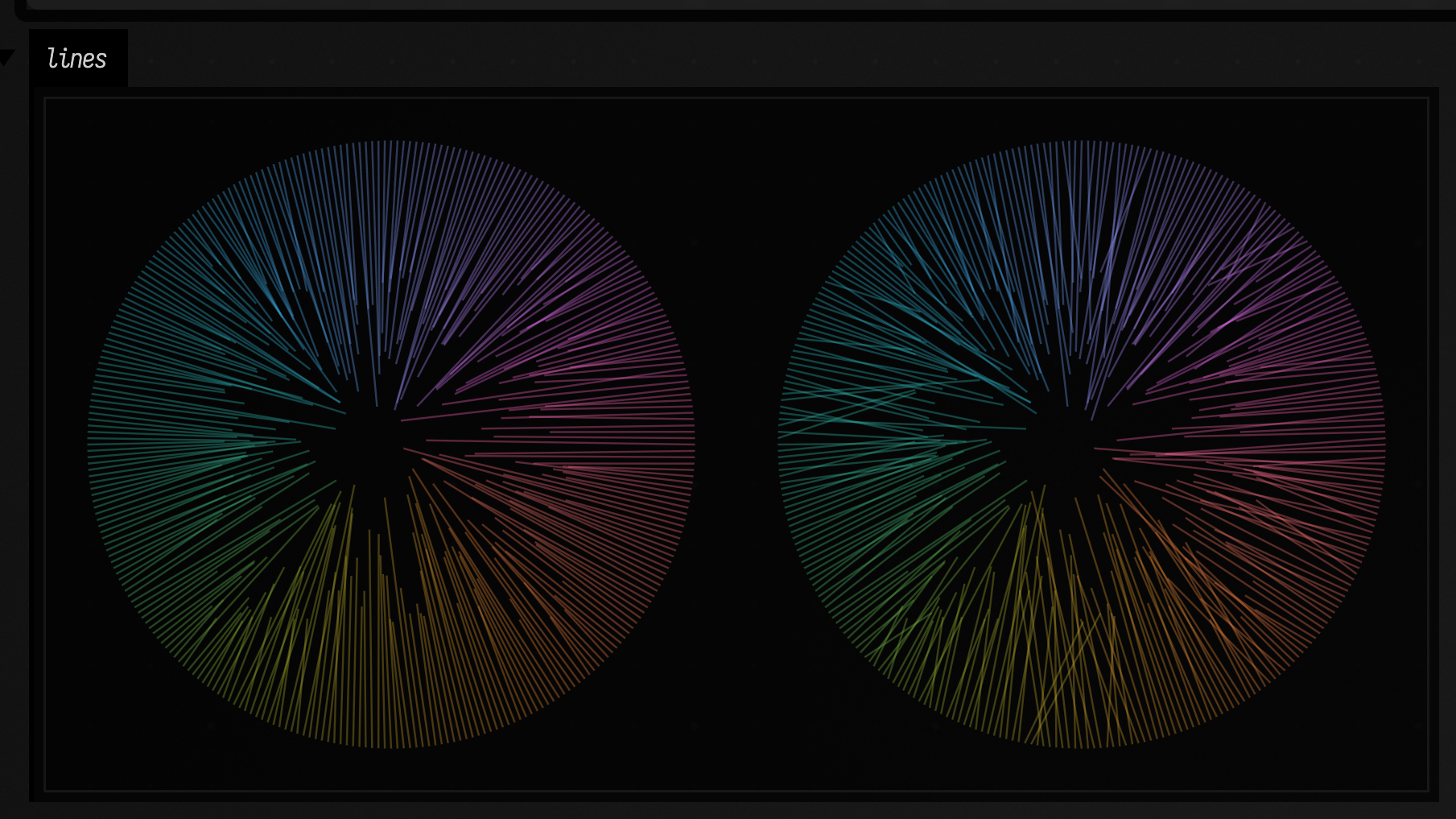

The exact matching's mean squared travel is the smallest possible, 15948 here, and BSP-OT's is 16083, under one percent above it; the crossing chords on the right are where the difference is.

assignment(cost) takes a cost matrix instead of points, for any cost you can compute: cost[i][j] is the price of sending source i to target j, and the matrix must be square.

Moving mass: Sinkhorn

sinkhorn relaxes both of the one-to-one rules. The two sets can be different sizes, each point can carry a weight, and a source can split between several targets. What comes back is a TransportPlan: plan.plan[i][j] is how much of source i goes to target j, every row adds up to that source's weight and every column to that target's, and the total cost plan.cost is as small as it can be subject to one more term, the entropy of the plan, scaled by epsilon. That term is what makes the problem fast and smooth to solve, and it is also a dial: a large epsilon blurs each source over many targets, and a small one makes the plan nearly a one-to-one matching.

epsilon is in the units of the cost, and with squared distances that is an area: its square root is roughly how far the blur reaches. Here 40 weighted points in a blob send their mass to 25 on a ring, at epsilon = 5000 on the left and 50 on the right; each line's brightness is how much moves along it, and each blob point's size is its weight:

// 40 points in a blob, weighted toward its top, and 25 evenly spaced on a ring beside it.
// Sinkhorn moves the mass of one onto the other; a line's brightness is how much moves along it.
val rnd = java.util.Random(5)
val blob = List(40) { vec(rnd.nextGaussian() * 25 - 110, rnd.nextGaussian() * 40) }
val ring = List(25) {
    val a = 2 * PI * it / 25
    vec(90 + 60 * cos(a), 60 * sin(a))
}
// the drawing's y runs down, so this makes the top of the blob heavier
val weights = DoubleArray(blob.size) { (1.0 - blob[it].y / 40.0).coerceAtLeast(0.1) }

fun dot(p: Vec2, dx: Double, r: Double) = FLine().circle(p.x + dx, p.y, r).also {
    it.filled = true
    it.stroked = false
    it.color = vec(0.8, 0.85, 0.95, 1.0)
}

fun panel(epsilon: Double, dx: Double): List<FLine> {
    val plan = sinkhorn(blob, ring, epsilon, sourceWeights = weights)
    println("ε = " + epsilon + ": " + plan)
    val most = plan.plan.maxOf { it.max() }
    val moves =
        blob.indices.flatMap { i ->
            ring.indices
                .filter { j -> plan.plan[i][j] > most * 0.02 }
                .map { j ->
                    FLine().moveTo(blob[i].x + dx, blob[i].y).lineTo(ring[j].x + dx, ring[j].y).also {
                        it.thickness = 1.2
                        it.color = vec(0.95, 0.72, 0.25, plan.plan[i][j] / most)
                    }
                }
        }
    return moves +
        blob.indices.map { dot(blob[it], dx, 1.5 + 2.5 * weights[it] / weights.max()) } +
        ring.map { dot(it, dx, 2.5) }
}

// ε is an area in the points' units: 5000 blurs over about √5000 ≈ 70, 50 over about 7
lines(panel(5000.0, -230.0) + panel(50.0, 230.0), w = 1000.0, h = 360.0, fitToSize = true)
displayOpen("lines")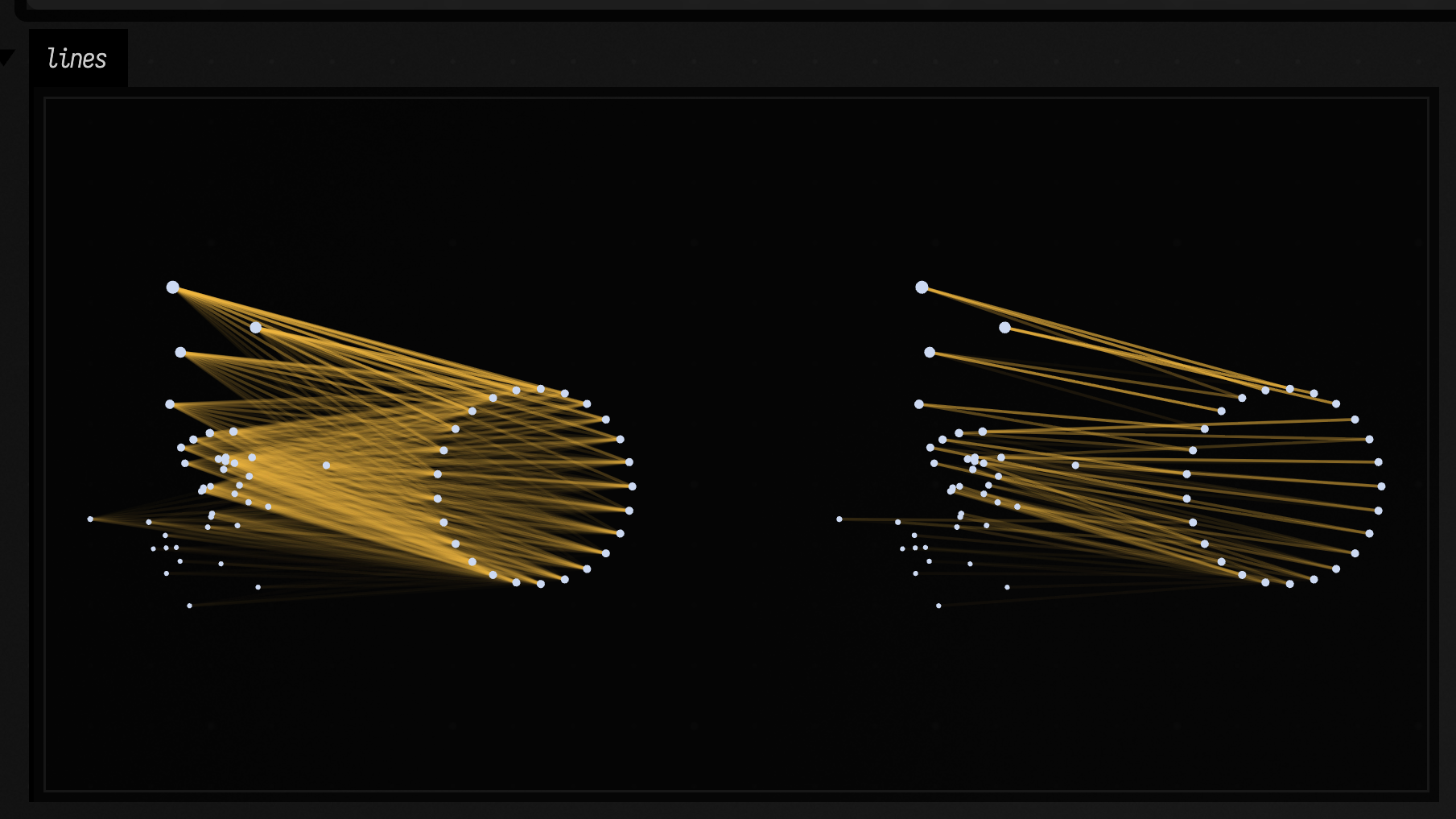

The plan's toString reports its cost, how many iterations it took and how far its marginals are from the weights. Smaller epsilon takes more iterations: here 20 at 5000 and 5200 at 50. As epsilon shrinks, the cost approaches the exact assignment cost. For equal sizes and weights, strongest() shows the target receiving the most mass from each source; inspect the full plan when you need a one-to-one assignment.

Two things to do with a plan:

• plan.barycentricMap(to) gives each source the weighted mean of the targets it sends mass to: where it goes, on average. With a small epsilon that is close to its single partner, so it is a way to move points that copes with the sets being different sizes.
• plan.f and plan.g are the dual potentials. The plan is \( \exp\bigl((f_i + g_j - \mathrm{cost}_{ij}) / \varepsilon\bigr) \), so they are a compact description of it, and sinkhorn(..., initialF = f, initialG = g) starts a new solve from them.

For a few thousand points or more, multiscaleSinkhorn solves a coarse version of the problem first, on centres chosen by farthest-point sampling, and starts each finer level from the potentials of the one before. The finest level is the full problem, so it reaches the plan sinkhorn would; it just takes fewer sweeps over the full-size cost matrix to get there.

How different are two distributions?

sinkhornDivergence(a, b, epsilon) turns transport into a number that says how far apart two weighted point sets are. It is the regularised cost of moving a onto b, minus half the cost of moving each onto itself, which removes the blur's own contribution: the divergence is zero when the sets are the same, and close to the real transport cost when they are not. A cloud shifted by t costs \( t^2 \) to move back:

// The Sinkhorn divergence between a cloud and the same cloud shifted by t is close to t²,
// the cost of moving it, and is zero at t = 0
val rnd = java.util.Random(7)
val cloud = List(60) { vec(rnd.nextGaussian() * 30, rnd.nextGaussian() * 30) }
val rows =
    [0.0, 5.0, 10.0, 20.0].map { t ->
        val shifted = cloud.map { vec(it.x + t, it.y) }
        val divergence = sinkhornDivergence(cloud, shifted, epsilon = 25.0)
        "shift $t: divergence ${divergence.f2}, t² = ${t * t}"
    }
display("divergence", rows.joinToString("<br>"))
displayOpen("divergence")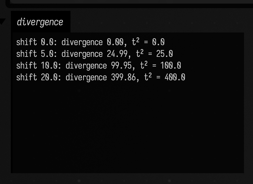

Unlike a distance between means or histograms, this compares the shapes of the two clouds as well as where they sit, and it is smooth in the point positions, which is why it is a common training loss for generated point clouds.