State estimation: tracking what you cannot measure

Some quantities you care about are never observed directly. You see a noisy position but want the velocity; you see one coordinate of a chaotic system but need its hidden delayed state; you have a measurement but not the model parameter that produced it. State estimation is the machinery for recovering the hidden value — and its uncertainty — from a stream of noisy, partial measurements.

pf.kt in the standard library gives you two tools for this:

UnscentedKalmanFilter — a nonlinear filter for continuous state (up to 3 dimensions). You hand it your own transition and observation functions as plain Kotlin lambdas; it never asks you to derive a Jacobian by hand the way an extended Kalman filter would.
UKFParticleFilter — a bank of particles, each carrying its own UKF plus a hypothesis about the model (an unknown parameter, a discrete mode). It keeps several explanations of the data alive at once and lets the measurements decide which survive.

These examples use Field's Plotly bridge: a Plot goes straight to an output with display(plot), so the truth, the measurement, and the estimate all land in the same frame.

The unscented Kalman filter

The shape of the API

The filter carries a mean state x (a DoubleArray) and a covariance p (a Matrix, which is just typealias Matrix = Array<DoubleArray>). You construct it with an initial guess and an initial covariance, then alternate two calls:

val ukf = UnscentedKalmanFilter(
    initialState = doubleArrayOf(1.0, 0.96, 0.92), // your best initial guess
    initialCovariance = diag(0.08, 0.08, 0.08), // how unsure you are of it
    options = UKFOptions(alpha = 0.55),
)

ukf.predict(processNoise = diag(0.004, 0.004, 0.004)) { state ->
    // where does the state go on its own, over one step?
    advance(state)
}

ukf.update(
    measurement = doubleArrayOf(y),
    measurementNoise = diag(0.05 * 0.05),
) { state ->
    // what would this state look like through your sensor?
    doubleArrayOf(state[0])
}

val estimate = ukf.stateCopy() // read the mean; covarianceCopy() reads p

predict pushes the state forward through your transition lambda and inflates the covariance by processNoise. update corrects the state toward a measurement, trusting it in proportion to measurementNoise. The observe lambda maps a full state to what your sensor would report; here it exposes only state[0], so the filter estimates the other coordinates purely from the dynamics.

Two constraints come straight from pf.kt: the state dimension must be 1–3 and the measurement dimension must be 1–3. The two do not have to match.

The `UKFOptions` knobs

UKFOptions controls how the filter picks its sigma points — the small set of sample states it propagates through your nonlinear functions to estimate the new mean and covariance:

field	default	what it does
`alpha`	`0.5`	spread of the sigma points around the mean. Small `alpha` clusters them tight (good for mild nonlinearity); larger `alpha` spreads them out. Must be `> 0`.
`beta`	`2.0`	folds prior knowledge of the distribution into the covariance weight. `2.0` is optimal for Gaussians and is almost always the right choice.
`kappa`	`0.0`	secondary scaling. Usually left at `0`; raise it if the sigma-point scale \( n + \lambda \) would otherwise go non-positive.
`jitter`	`1e-9`	tiny diagonal added when a covariance is not quite positive-definite, so the internal Cholesky step stays numerically safe. Must be `> 0`.

alpha is the knob you actually reach for. The examples below use alpha = 0.55 and alpha = 0.9; if you ever see "n + lambda must be positive", nudge alpha or kappa up.

Diagonal matrices: `diag`

Matrix values are just arrays of arrays, so covariance matrices are easy to build inline, and diag(0.1, 0.1, 0.5) makes a diagonal one.

The Gaussian noise the examples inject comes from the standard-library randomGaussian() (a zero-mean, unit-variance draw).

Example: tracking a hidden Mackey-Glass point

In this first example one hidden point moves through a nonlinear delayed map (the Mackey-Glass system). The only measurement is that point plus Gaussian error, and the UKF predicts the motion, then corrects it from that one number. The state carries three coordinates (the current value and two delayed ones), but only the first is ever observed.

:::static
import space.kscience.plotly.*

fun mackeyGlassStep(state: DoubleArray, beta: Double = 0.28): DoubleArray {
    val x = state[0].coerceIn(0.02, 3.0)
    val delayed = state[2].coerceIn(0.02, 3.0)
    val dx = beta * delayed / (1.0 + delayed.pow(10.0)) - 0.10 * x
    val next = (x + dx).coerceIn(0.02, 3.0)
    return doubleArrayOf(next, x, state[1])
}

val ukf = UnscentedKalmanFilter(
    initialState = doubleArrayOf(1.00, 0.96, 0.92),
    initialCovariance = diag(0.08, 0.08, 0.08),
    options = UKFOptions(alpha = 0.55),
)

val trueX = mutableListOf<Double>()
val measuredX = mutableListOf<Double>()
val estimatedX = mutableListOf<Double>()
var truth = doubleArrayOf(1.12, 1.05, 0.98)

repeat(360) { i ->
    val forcing = 0.020 * sin(i * 0.045)
    truth = mackeyGlassStep(truth, beta = 0.20 + forcing)
    truth[0] = (truth[0] + 0.003 * randomGaussian()).coerceIn(0.02, 3.0)

    val measurement = truth[0] + 0.006 * randomGaussian()

    ukf.predict(processNoise = diag(0.004, 0.004, 0.004)) { state ->
        mackeyGlassStep(state, beta = 0.20)
    }
    ukf.update(
        measurement = doubleArrayOf(measurement),
        measurementNoise = diag(0.05 * 0.05),
    ) { state ->
        doubleArrayOf(state[0])
    }

    trueX += truth[0]
    measuredX += measurement
    estimatedX += ukf.stateCopy()[0]
}

val sample = trueX.indices.toList()
val plot =
    Plotly.plot {
            trace {
                name = "measurement"
                x.set(sample)
                y.set(measuredX)
                line.width = 0.1
            }
            trace {
                name = "hidden x"
                x.set(sample)
                y.set(trueX)
                line.width = 0.5
            }
            trace {
                name = "UKF estimate"
                x.set(sample)
                y.set(estimatedX)
                line.width = 1.0
            }
            layout {
                title = "UKF tracking a noisy Mackey-Glass point"
                xaxis {
                    title = "time step"
                }
                yaxis {
                    title = "x"
                }
            }
        }
        .darkMode()

display(plot)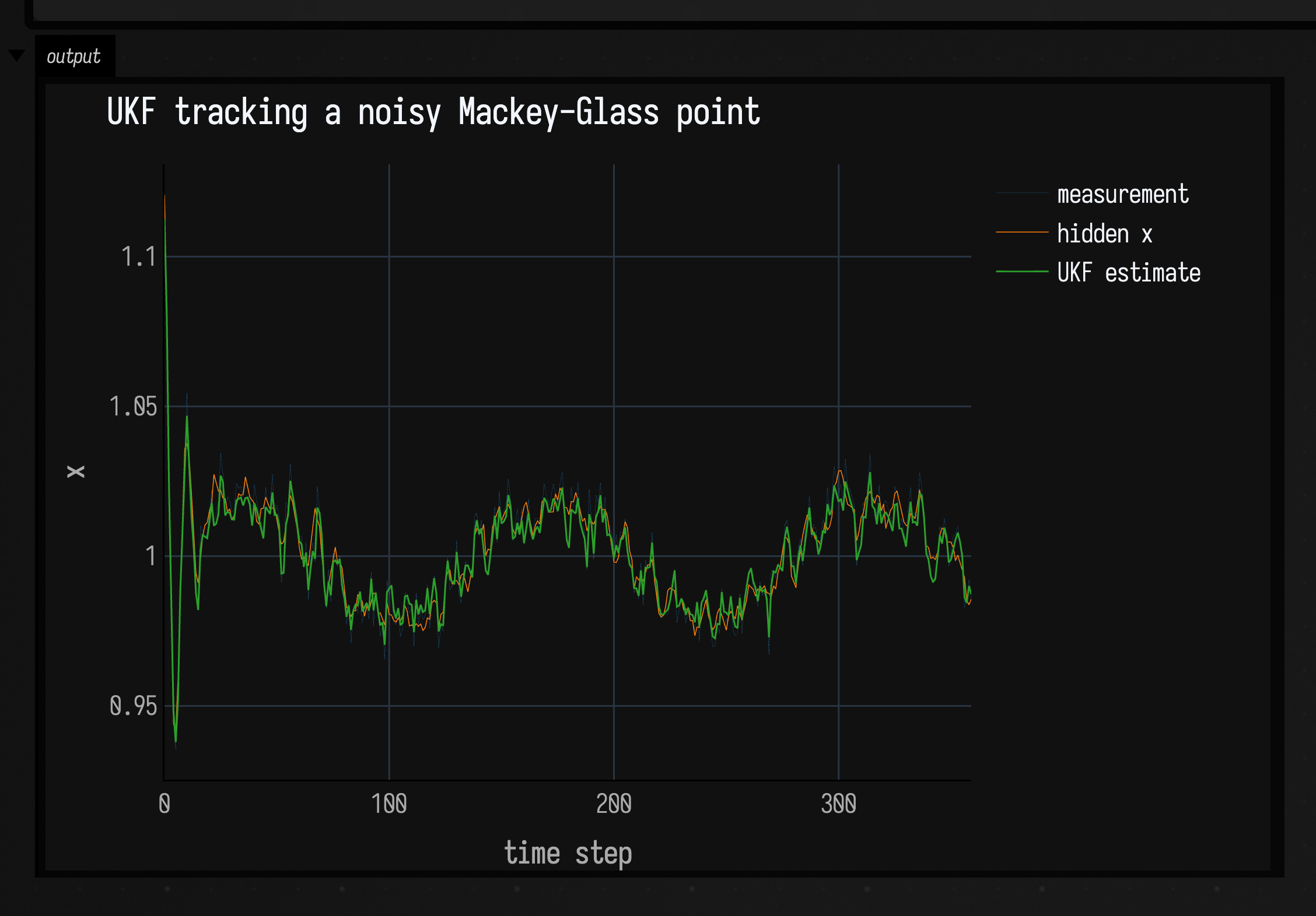

A UKF estimate following a noisy hidden Mackey-Glass point

The measurement jitters around the hidden state while the UKF estimate follows the nonlinear trend without chasing every sample. Note that the observation model returns only state[0] while the filter still carries the delayed coordinates it needs to predict.

Example: recovering an unmeasured velocity

In the Mackey-Glass example the unobserved coordinates were only needed to predict. Here the unobserved value is the one you want: the state is [position, velocity], the sensor reports only a noisy position, and the filter has to infer velocity from how the position moves. A constant-velocity transition (position += velocity·dt) plus a little process noise on the velocity lets the estimate follow a trajectory that curves.

:::static
import space.kscience.plotly.*

// State = [position, velocity]. We measure only a noisy position; velocity is
// never observed and must be reconstructed from the dynamics.
val dt = 1.0
val ukf = UnscentedKalmanFilter(
    initialState = doubleArrayOf(0.0, 0.0),
    initialCovariance = diag(1.0, 1.0),
    options = UKFOptions(alpha = 0.9),
)

val truePos = mutableListOf<Double>()
val trueVel = mutableListOf<Double>()
val measuredPos = mutableListOf<Double>()
val estPos = mutableListOf<Double>()
val estVel = mutableListOf<Double>()

var pos = 0.0
repeat(220) { i ->
    // True velocity follows a slow sine, so position curves rather than drifts.
    val vel = 1.2 * sin(i * 0.03)
    pos += vel * dt

    val measurement = pos + 3.0 * randomGaussian() // noisy POSITION only

    // Constant-velocity model: position advances by velocity, velocity coasts.
    ukf.predict(processNoise = diag(0.01, 0.05)) { s ->
        doubleArrayOf(s[0] + s[1] * dt, s[1])
    }
    ukf.update(
        measurement = doubleArrayOf(measurement),
        measurementNoise = diag(3.0 * 3.0),
    ) { s ->
        doubleArrayOf(s[0]) // the sensor sees position, not velocity
    }

    val x = ukf.stateCopy()
    truePos += pos
    trueVel += vel
    measuredPos += measurement
    estPos += x[0]
    estVel += x[1]
}

val sample = truePos.indices.toList()

val positionPlot =
    Plotly.plot {
            trace {
                name = "measured position"
                x.set(sample)
                y.set(measuredPos)
                line.width = 0.3
            }
            trace {
                name = "true position"
                x.set(sample)
                y.set(truePos)
                line.width = 1.5
            }
            trace {
                name = "UKF position"
                x.set(sample)
                y.set(estPos)
                line.width = 1.0
            }
            layout {
                title = "Position: measured vs true vs estimated"
                xaxis { title = "time step" }
                yaxis { title = "position" }
            }
        }
        .darkMode()

val velocityPlot =
    Plotly.plot {
            trace {
                name = "true velocity"
                x.set(sample)
                y.set(trueVel)
                line.width = 1.5
            }
            trace {
                name = "UKF velocity (never measured)"
                x.set(sample)
                y.set(estVel)
                line.width = 1.0
            }
            layout {
                title = "Velocity is recovered from position alone"
                xaxis { title = "time step" }
                yaxis { title = "velocity" }
            }
        }
        .darkMode()

display("position", positionPlot)
display("velocity", velocityPlot)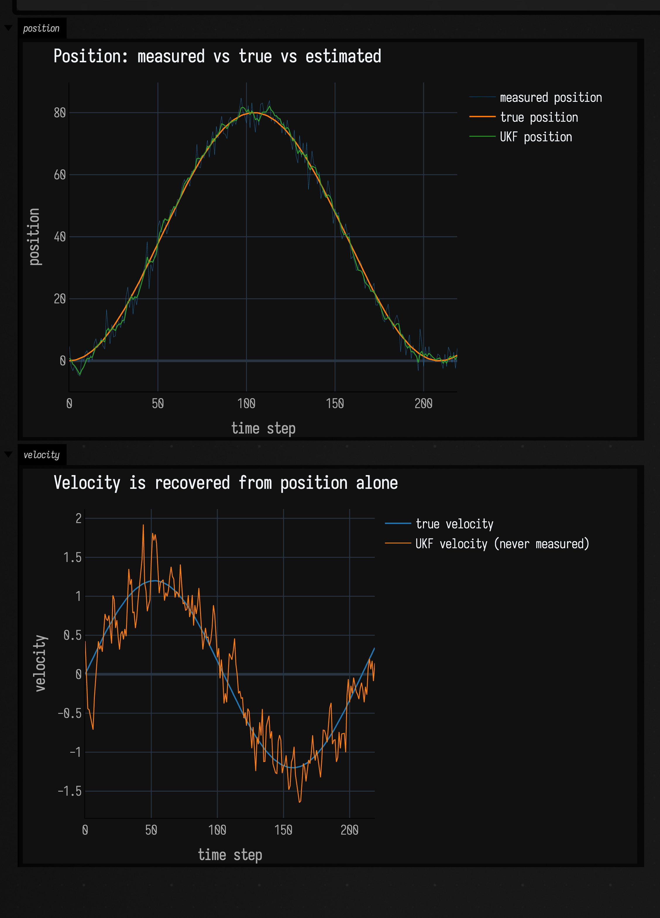

A UKF recovering an unmeasured velocity from noisy position measurements

The top panel compares the noisy measurement with the estimate. In the bottom panel the estimated velocity follows the true sine, although velocity is never measured.

The particle filter: keeping several models alive

The UKF assumes you know the model. When the system itself is uncertain (an unknown parameter, a regime that can switch), reach for UKFParticleFilter. Each particle is a UKFParticle pairing a UnscentedKalmanFilter with a hypothesis of type H and a logWeight:

UKFParticle(
    ukf = UnscentedKalmanFilter(/* ... */ ),
    hypothesis = MackeyGlassHypothesis(beta = 0.3),
    logWeight = 0.0,
)

The filter's cycle mirrors the UKF's, but every lambda now also receives the particle's hypothesis, and processNoise / measurementNoise are functions of the particle so each can carry its own:

predict(processNoise, transition, evolveHypothesis) — advances each particle's UKF using transition(hypothesis, state); the optional evolveHypothesis lets the hypotheses drift or occasionally jump.
update(measurement, measurementNoise, observe) — corrects each UKF and reweights particles by how well they explained the measurement.
resampleIfNeeded(thresholdFraction, random, roughening) — when the effective sample size drops below a fraction of the population, resamples toward the likely particles and (optionally) roughens them via RougheningOptions so the cloud does not collapse to identical clones.
estimateMean() / estimateCovariance() read the weighted state; weights() and effectiveSampleSize() expose the particle health; roughenHypotheses perturbs the discrete/parameter part of each hypothesis.

Here each particle carries a different Mackey-Glass beta, the measurements see the current point plus the two previous ones, and the weights gradually favour the beta whose dynamics explain the data. Partway through, the true beta jumps, and the cloud has to find it again from a population that had already settled.

:::static
import kotlin.random.Random
import space.kscience.plotly.*
import space.kscience.plotly.models.Dash
import space.kscience.plotly.models.ScatterMode

data class MackeyGlassHypothesis(val beta: Double)
data class ParticleSnapshot(
    val step: Int,
    val beta: List<Double>,
)

fun mackeyGlassStep(state: DoubleArray, beta: Double): DoubleArray {
    val x = state[0].coerceIn(0.02, 3.0)
    val delayed = state[2].coerceIn(0.02, 3.0)
    val dx = beta * delayed / (1.0 + delayed.pow(10.0)) - 0.10 * x
    val next = (x + dx).coerceIn(0.02, 3.0)
    return doubleArrayOf(next, x, state[1])
}

val rng = Random(31)
val particleCount = 96
val particles =
    (0 until particleCount).map { i ->
        val beta = 0.08 + 0.76 * i.toDouble() / (particleCount - 1).toDouble()
        UKFParticle(
            ukf = UnscentedKalmanFilter(
                initialState = doubleArrayOf(
                    0.80 + 0.18 * rng.nextGaussian(),
                    0.80 + 0.18 * rng.nextGaussian(),
                    0.80 + 0.18 * rng.nextGaussian(),
                ),
                initialCovariance = diag(0.35, 0.35, 0.35),
                options = UKFOptions(alpha = 0.55),
            ),
            hypothesis = MackeyGlassHypothesis(beta),
            logWeight = 0.0,
        )
    }

val pf = UKFParticleFilter<MackeyGlassHypothesis>(
    initialParticles = particles,
    copyHypothesis = { it.copy() },
)

fun betaEstimate(): Double {
    val weights = pf.weights()
    return pf.particles.indices.sumOf { i -> weights[i] * pf.particles[i].hypothesis.beta }
}

fun betaStdDev(mean: Double): Double {
    val weights = pf.weights()
    val variance =
        pf.particles.indices.sumOf { i ->
            val d = pf.particles[i].hypothesis.beta - mean
            weights[i] * d * d
        }
    return sqrt(variance)
}

val trueX = mutableListOf<Double>()
val measuredX = mutableListOf<Double>()
val estimatedX = mutableListOf<Double>()
val trueBeta = mutableListOf<Double>()
val estimatedBeta = mutableListOf<Double>()
val betaSigma = mutableListOf<Double>()
val particleSnapshots = mutableListOf<ParticleSnapshot>()
val snapshotSteps = setOf(0, 350, 700, 1055, 1200, 1600, 2200, 2800, 3199)

var truth = doubleArrayOf(1.10, 1.08, 1.05)
var lastMeasurement = truth[1]
var olderMeasurement = truth[2]
repeat(3200) { i ->
    val baseBeta = if (i < 1055) 0.23 else 0.64
    val actualBeta = baseBeta + 0.006 * sin(i * 0.037)

    truth = mackeyGlassStep(truth, actualBeta)
    truth[0] = (truth[0] + 0.006 * rng.nextGaussian()).coerceIn(0.00, 3.0)
    val measurement = truth[0] + 0.006 * rng.nextGaussian()

    pf.predict(
        processNoise = { diag(0.003, 0.003, 0.003) },
        transition = { hypothesis, state ->
            mackeyGlassStep(state, hypothesis.beta)
        },
        evolveHypothesis = { hypothesis ->
            val broadProposalRate = if (i in 980..1240) 0.004 else 0.00025
            val beta = if (rng.nextDouble() < broadProposalRate) {
                0.05 + 0.85 * rng.nextDouble()
            } else {
                    hypothesis.beta + 0.0002 * rng.nextGaussian()
                }
            hypothesis.copy(beta = beta.coerceIn(0.0, 1.0))
        },
    )
    pf.update(
        measurement = doubleArrayOf(measurement, lastMeasurement, olderMeasurement),
        measurementNoise = { diag(0.010 * 0.010, 0.014 * 0.014, 0.018 * 0.018) },
        observe = { _, state -> doubleArrayOf(state[0], state[1], state[2]) },
    )

    olderMeasurement = lastMeasurement
    lastMeasurement = measurement

    val resampled = pf.resampleIfNeeded(
        thresholdFraction = 0.55,
        random = rng,
        roughening = RougheningOptions(factor = 0.012, minimumStdDev = 1e-5),
    )
    if (resampled) {
        val centerBeta = betaEstimate()
        pf.roughenHypotheses(rng) { hypothesis, random ->
            val contracted = centerBeta + 0.82 * (hypothesis.beta - centerBeta)
            hypothesis.copy(beta = (contracted + 0.0007 * random.nextGaussian()).coerceIn(0.0, 1.0))
        }
    }

    trueX += truth[0]
    measuredX += measurement
    estimatedX += pf.estimateMean()[0]
    trueBeta += actualBeta
    val betaMean = betaEstimate()
    estimatedBeta += betaMean
    betaSigma += betaStdDev(betaMean)
    if (i in snapshotSteps) {
        particleSnapshots +=
            ParticleSnapshot(
                step = i,
                beta = pf.particles.map { it.hypothesis.beta },
            )
    }
}

val sample = trueX.indices.toList()

// Over all 3,200 steps the oscillation is a solid block, so show 100 steps of it.
val window = (1000 until 1100).toList()
val statePlot =
    Plotly.plot {
            layout {
                title = "State tracking, steps 1000 to 1100"
                xaxis { title = "time step" }
            }
            scatter {
                name = "measurement"
                x.set(window)
                y.set(window.map { measuredX[it] })
                mode = ScatterMode.markers
                marker { size = 4.0 }
            }
            trace {
                name = "hidden x"
                x.set(window)
                y.set(window.map { trueX[it] })
                line.width = 2.0
            }
            trace {
                name = "PF estimate"
                x.set(window)
                y.set(window.map { estimatedX[it] })
                line.width = 1.5
                line.dash = Dash.dash
            }
        }
        .darkMode()

val betaPlot =
    Plotly.plot {
            trace {
                name = "true beta"
                x.set(sample)
                y.set(trueBeta)
                line.width = 1.5
            }
            trace {
                name = "particle beta estimate"
                x.set(sample)
                y.set(estimatedBeta)
                line.width = 0.5
            }
            trace {
                name = "estimate + weighted sd"
                x.set(sample)
                y.set(estimatedBeta.indices.map { estimatedBeta[it] + betaSigma[it] })
                line.width = 0.6
            }
            trace {
                name = "estimate - weighted sd"
                x.set(sample)
                y.set(estimatedBeta.indices.map { estimatedBeta[it] - betaSigma[it] })
                line.width = 0.6
            }
        }
        .darkMode()

val particlePlot =
    Plotly.plot {
            layout {
                title = "Particle beta hypotheses over time"
                xaxis {
                    title = "time step"
                }
                yaxis {
                    title = "beta hypothesis"
                }
            }
            particleSnapshots.forEach { snapshot ->
                scatter {
                    name = "t=${snapshot.step}"
                    x.set(List(snapshot.beta.size) { snapshot.step })
                    y.set(snapshot.beta)
                    mode = ScatterMode.markers
                    marker {
                        size = 4.0
                        opacity = 0.28
                    }
                }
            }
            trace {
                name = "true beta"
                x.set(sample)
                y.set(trueBeta)
                line.width = 2.0
            }
            trace {
                name = "weighted estimate"
                x.set(sample)
                y.set(estimatedBeta)
                line.width = 2.0
            }
        }
        .darkMode()

display("state tracking", statePlot)
display("model estimate", betaPlot)
display("particles", particlePlot)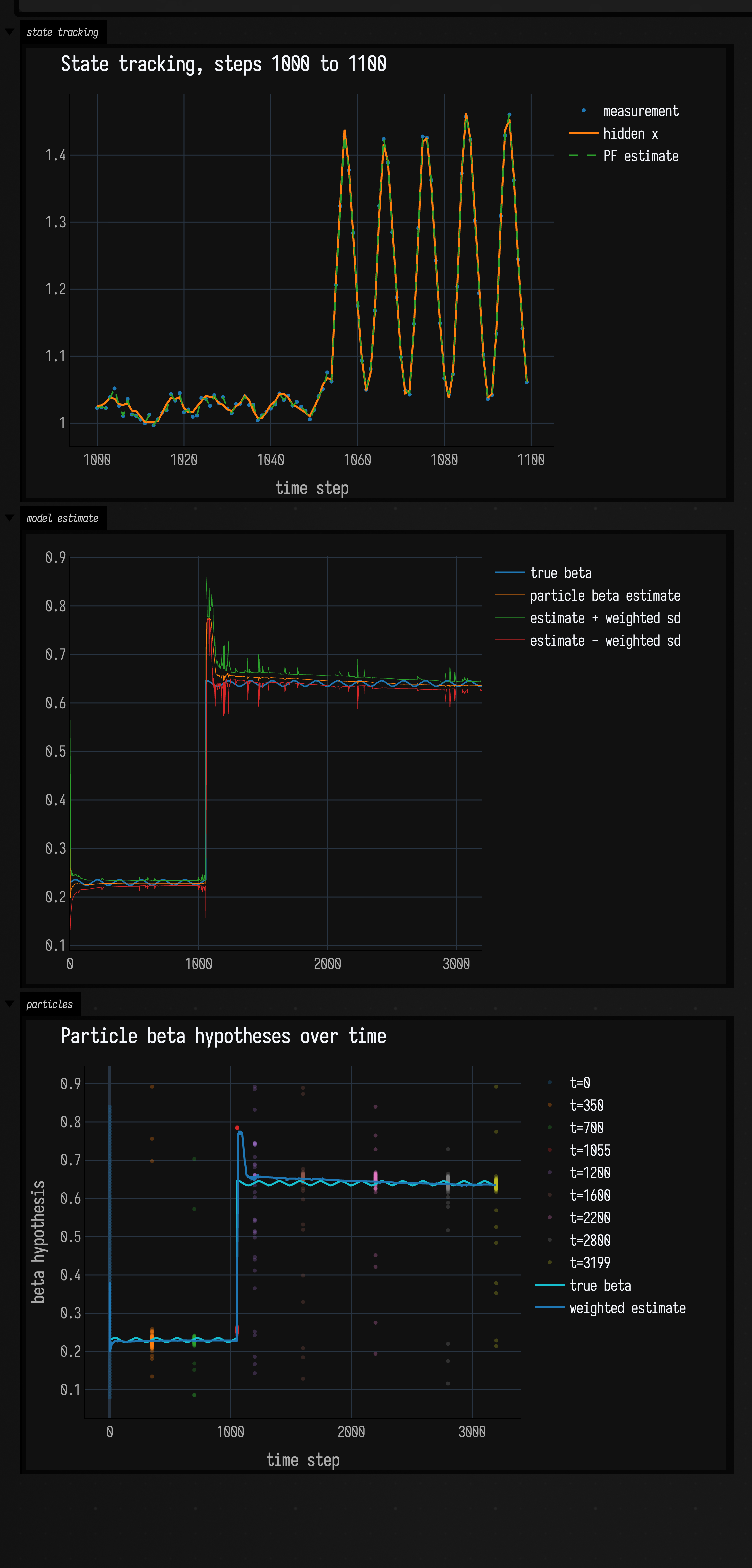

Particle-filter panels. The top one zooms to steps 1000 to 1100: the hidden x wobbles near 1.02, then jumps into an oscillation between 1.0 and 1.45 when beta changes, and the dashed PF estimate stays on it with the measurement dots scattered around both. Below, the beta estimate with a weighted envelope, and the particle beta cloud over time

The state panel shows 100 steps around the change in beta, since all 3,200 steps of the oscillation would draw as a solid block; the beta panel shows the true beta, the weighted particle estimate, and a weighted one-standard-deviation envelope; the particle panel scatters each hypothesis at saved time steps, and because the markers are translucent, a bright saturated band is where the particles have clumped and loose dots are where they have not.

Observing the current point plus the two previous measurements pins the delayed state coordinates, so a wrong beta cannot hide behind a different latent delay. The broad-proposal rate is raised only around the known transition window: enough diversity to catch the jump, without repopulating far-away hypotheses once the estimate has settled.

For raw and filtered signals rather than these derived quantities, continue with the time-domain signal examples; for interpolation, keyframes, and correlation, see Values over time.

The public declarations used on this page are listed, with their KDoc, in the codebase reference: pf.kt. Start from what's already in the box.