Projecting a distance matrix
Suppose you have a set of things and one number for each pair: how far apart they are. Twenty words and an edit distance. A hundred and
sixty samples along a curve and the number of hops between them. A thousand mel frames and a
Wasserstein distance. There is nothing to plot, because the things have no coordinates, which is the
whole problem, and it is what smile_mds.kt is for. Give it the distances and it
invents coordinates that reproduce them as closely as two dimensions allow.
Two of the functions take vectors and compute the distances for you, which is what the speech-embedding and short-time spectral pages use. The other two take a distance matrix you computed yourself: transport, edit and graph distances, or anything else you can measure between two things. Both examples below build their own matrix.
On Apple Silicon the eigensolver is LAPACK
smileMds probes the ARPACK binding once and falls back to LAPACK's dsyevd when it is
missing (smile_mds.kt:349). On macosx-arm64
it is missing: the ARPACK native library this build pins wants a Fortran runtime that no
bytedeco artifact ships for that platform
(build.gradle.kts:119). So LAPACK is the path the numbers
on this page were measured on. smileTsne does not touch ARPACK either way.
Where the family lives
| what you have | what to call | what comes back |
|---|---|---|
| equal-length vectors, and you want cosine or Euclidean distance computed for you | smileMds (smile_mds.kt:88) |
SmileMdsProjection — coordinates, scores, stress1, distanceCorrelation |
| a symmetric distance matrix you built yourself | smileMdsDistances (smile_mds.kt:159) |
SmileMdsProximityProjection — the same three, plus the label you passed |
| vectors, but you care about local neighbourhoods rather than global geometry | smileTsne (smile_mds.kt:180) |
SmileTsneProjection — coordinates, cost, seed |
| your own matrix, t-SNE | smileTsneDistances (smile_mds.kt:240) |
SmileTsneProximityProjection |
SmileMdsDistance is COSINE or EUCLIDEAN and only matters to the two vector-taking calls; the
matrix-taking calls never see your vectors at all, which is exactly why they accept a distance no
vector could express.
Some limits first. None of these projections is invertible, and none can
place a new point without refitting everything, so this is not dimensionality reduction for a model.
Nothing here assigns labels either: a picture with visible clumps is a picture, not a partition. And
none of it is cheap at scale, because the proximity matrix is \( n^2 \) doubles
(smile_mds.kt:111), 191 MiB at
5000 rows and 3.0 GiB at 20 000, before Smile allocates its own.
A distance you wrote yourself
Twenty words, four families of five: compute/computes/computed/computer/computing, then
the same five shapes on render, listen and sample. The distance is Levenshtein: the number of
single-character insertions, deletions and substitutions between two strings. There is no vector
anywhere; a word is not a point in any space until this call gives it one.
:::static
import space.kscience.plotly.*
import space.kscience.plotly.models.ScatterMode
import space.kscience.plotly.models.TextPosition

val families = [
    ["compute", "computes", "computed", "computer", "computing"],
    ["render", "renders", "rendered", "renderer", "rendering"],
    ["listen", "listens", "listened", "listener", "listening"],
    ["sample", "samples", "sampled", "sampler", "sampling"],
]
val words = families.flatten()

/*
Ordinary Levenshtein, in the fence rather than from the stdlib: `afield.lang.brief.editDistance`
exists but is `internal`, and naming a doc-local helper after a stdlib symbol would put a false
"Used in" back-reference in the generated reference.
*/
val wordEditDistance = { a: String, b: String ->
    var previous = IntArray(b.length + 1) { it }
    for (i in 1..a.length) {
        val current = IntArray(b.length + 1)
        current[0] = i
        for (j in 1..b.length) {
            val substitution = previous[j - 1] + if (a[i - 1] == b[j - 1]) 0 else 1
            current[j] = minOf(previous[j] + 1, current[j - 1] + 1, substitution)
        }
        previous = current
    }
    previous[b.length]
}

val distances =
    Array(words.size) { a ->
        DoubleArray(words.size) { b -> wordEditDistance(words[a], words[b]).toDouble() }
    }
val projection = smileMdsDistances(distances, dimensions = 2, label = "levenshtein")

// The plane distances used by the neighbour count below.
val plane =
    Array(words.size) { a ->
        DoubleArray(words.size) { b ->
            val dx = projection.coordinates[a][0] - projection.coordinates[b][0]
            val dy = projection.coordinates[a][1] - projection.coordinates[b][1]
            sqrt(dx * dx + dy * dy)
        }
    }

// The claim the picture makes, as a count rather than an impression: does each word's nearest
// neighbour still come from its own family?
val ownFamily = { matrix: Array<DoubleArray> ->
    words.indices.count { row ->
        val nearest = words.indices.filter { it != row }.minByOrNull { matrix[row][it] }!!
        nearest / 5 == row / 5
    }
}
val lost =
    words.indices
        .filter { row ->
            val nearest = words.indices.filter { it != row }.minByOrNull { plane[row][it] }!!
            nearest / 5 != row / 5
        }
        .map { words[it] }

val within = ArrayList<Double>()
val between = ArrayList<Double>()
for (a in words.indices) for (b in 0 until a) {
    if (a / 5 == b / 5) within += distances[a][b] else between += distances[a][b]
}
println(
    "input edit distance: within-family mean ${within.average().f3}, " +
        "between-family mean ${between.average().f3} (smallest between-family ${between.min()})",
)
println("retained eigenvalues ${projection.scores.joinToString { it.f3 }}")
println(
    "plane vs input: r = ${projection.distanceCorrelation.f4}, " +
        "stress-1 = ${projection.stress1.f4}",
)
println(
    "nearest neighbour in own family: ${ownFamily(distances)}/20 by edit distance, " +
        "${ownFamily(plane)}/20 in the plane; lost: $lost",
)
:::fold draw the twenty words
val palette = ["#7ad9ff", "#ff9e4a", "#8fff9a", "#c58cff"]
display(
    "plane",
    Plotly.plot {
            // Words in one family land close together, so each of the five puts its label on a
            // different side of its marker.
            val sides = [
                TextPosition.`top center`,
                TextPosition.`bottom center`,
                TextPosition.`middle right`,
                TextPosition.`middle left`,
                TextPosition.`top right`,
            ]
            families.forEachIndexed { family, members ->
                members.indices.forEach { i ->
                    val row = family * 5 + i
                    scatter {
                        name = members.first()
                        legendgroup = members.first()
                        showlegend = i == 0
                        mode = ScatterMode.`markers+text`
                        x.set([projection.coordinates[row][0]])
                        y.set([projection.coordinates[row][1]])
                        text.set([words[row]])
                        textposition = sides[i]
                        marker {
                            size = 9.0
                            color(palette[family])
                        }
                        textfont {
                            color(palette[family])
                            size = 13
                        }
                    }
                }
            }
            layout {
                title = "Twenty words placed by edit distance alone (classical MDS)"
                height = 1000 // tall, so labels inside a clump have room
                xaxis {
                    title = "coordinate 1"
                    range = -8.0..8.5 // room for the labels at either edge
                }
                yaxis { title = "coordinate 2" }
            }
        }
        .darkMode(),
)
:::endfold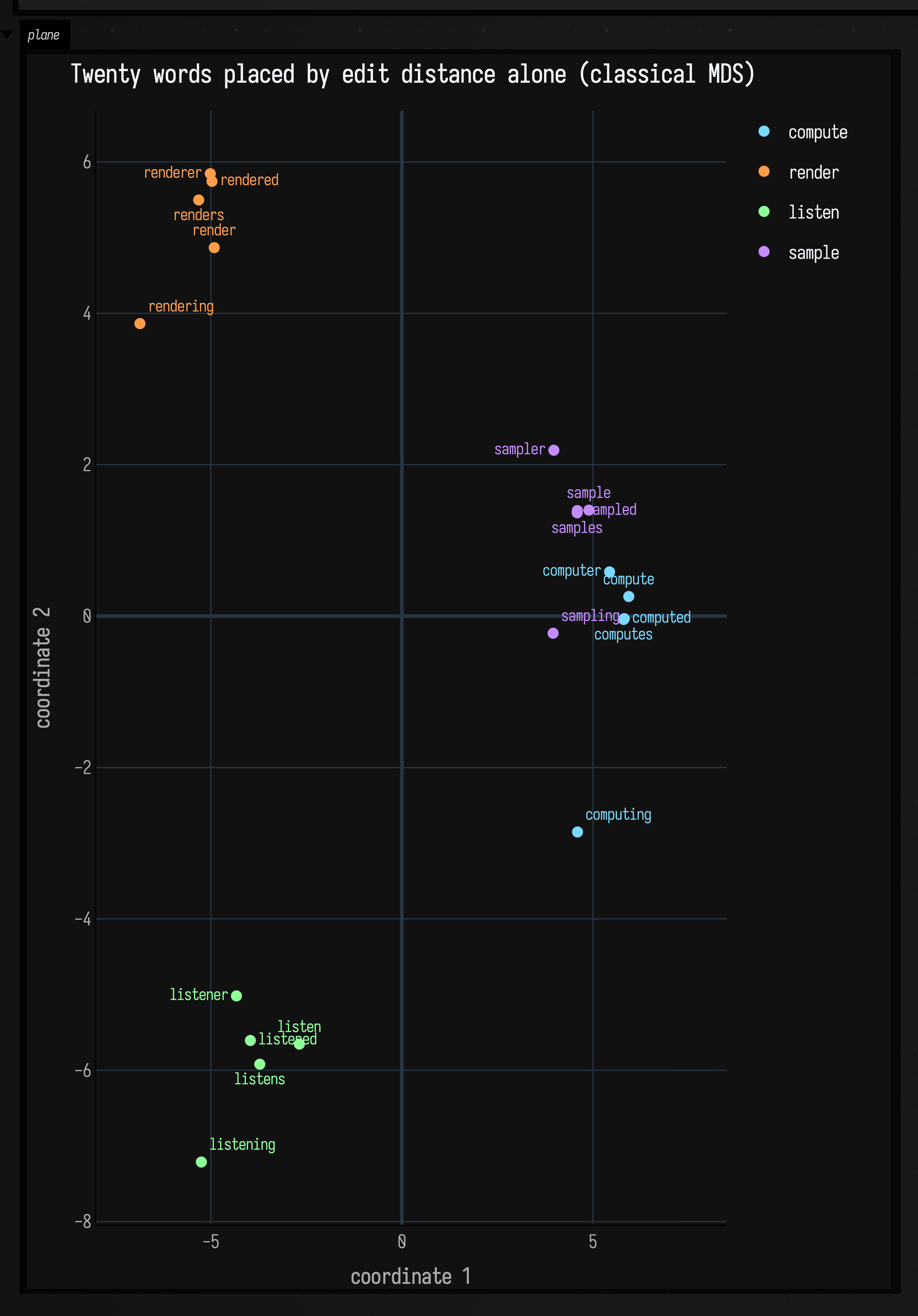
Read the numbers the fence prints rather than the shape. The mean edit distance inside a family is
2.000 and between families 6.720, so a reader would expect four clumps, and four clumps is
what appears. What the projection destroyed to get them is on the last line: by edit distance, all
20 of 20 words have a same-family nearest neighbour; in the plane, 18 of 20 do. The two that
lose it are computing and sampling, and the arithmetic behind that is the cost of a projection in
miniature. The compute and sample families are 4 apart form for form:
compute/sample, computed/sampled, computing/sampling, all exactly 4, and 4 is the smallest
between-family distance anywhere in the set. Meanwhile every -ing form is 3 from its own stem, the
largest within-family distance there is. So computing sits 3 from its family and 4 from sampling,
a margin of one, and one is what two dimensions cannot hold: in the plane its nearest neighbour is
sampling. sampling does worse still: its plane-nearest is computer, which is 6 away in the
input. Those are the two clumps that touch in the figure above, and they touch for a reason you can
read off the distance matrix before you draw anything.
The fit itself, which the projection reports as distanceCorrelation and stress1 (Kruskal's
stress-1 at the scale that minimises it, since classical MDS does not promise the plane is in the
input's units): the plane distances correlate with the edit distances at r = 0.8475, with a
stress-1 of 0.2780. Stress-1 above 0.2 is usually called poor, so that is a poor fit, and it is
what squeezing a nineteen-dimensional structure into two costs. Ask for more dimensions and it
improves the way you would expect: dimensions = 3 gives r = 0.9258 and stress 0.1547,
dimensions = 4 gives 0.9500 and 0.1146. Nothing forces you to draw all the dimensions you fit.
A graph distance: hop count on a KNN spiral
Take 160 points along a two-turn spiral, join each to its four
nearest neighbours with vec2KnnGraph (graph_connectivity.kt:584), and count
hops. That is a distance defined entirely by the graph: two points on adjacent arms of the spiral
are close in the plane and far apart along the curve, and hop count is the one that knows it.
Feed the hop matrix to smileMdsDistances and you have Isomap, a standard way of unrolling a curved
shape. The spiral also tells you whether it worked: each point has a true position along the curve,
and a good projection recovers a coordinate that rises steadily with it.
:::static
import space.kscience.plotly.*
import space.kscience.plotly.models.ScatterMode

val n = 160
val t = DoubleArray(n) { it / (n - 1.0) }
val xy =
    Array(n) { i ->
        val theta = 2.0 * PI * 2.0 * t[i]
        val radius = 0.18 + 0.62 * t[i]
        doubleArrayOf(radius * cos(theta), radius * sin(theta))
    }
val points = (0 until n).map { vec(xy[it][0], xy[it][1]) }

/*
k = 4 works here because the arms are further apart than the samples are: the radial gap between
successive turns is 0.62 / 2 = 0.310 and the mean spacing along the curve is 0.0389, eight times
smaller. The guard against a shortcut edge is printed below rather than assumed — an edge joining
two arms would join points far apart in index, and this graph's worst is 4.
*/
val graph = vec2KnnGraph(points, k = 4)
val adjacency = Array(n) { graph.neighbors(it).toIntArray() }

// Breadth-first hop counts from every point: an unweighted geodesic over the k-NN graph.
val hops =
    Array(n) { source ->
        val depth = IntArray(n) { -1 }
        depth[source] = 0
        val queue = ArrayDeque<Int>()
        queue += source
        while (queue.isNotEmpty()) {
            val at = queue.removeFirst()
            for (next in adjacency[at]) if (depth[next] < 0) {
                depth[next] = depth[at] + 1
                queue += next
            }
        }
        DoubleArray(n) { depth[it].toDouble() }
    }

val geodesic = smileMdsDistances(hops, dimensions = 2, label = "graph hops")
// The control: the same 160 points, projected from their ordinary straight-line distances. In two
// dimensions that can only give the spiral back, rotated.
val straight = smileMds(xy, dimensions = 2, distance = SmileMdsDistance.EUCLIDEAN, positiveCorrection = false)

// MDS axes have arbitrary sign, so orient both to agree with t before comparing them.
val orient = { coordinates: Array<DoubleArray> ->
    val raw = DoubleArray(n) { coordinates[it][0] }
    val sign = if (StatsDependence.spearman(t, raw) < 0.0) -1.0 else 1.0
    DoubleArray(n) { sign * raw[it] }
}
val geodesicAxis = orient(geodesic.coordinates)
val straightAxis = orient(straight.coordinates)

println(
    "graph: ${graph.edges.size} edges, worst |i - j| over an edge = ${graph.edges.maxOf { abs(it.i - it.j) }}" +
        " (a shortcut between arms would be large); diameter ${hops.maxOf { it.max() }.toInt()} hops",
)
println("coordinate 1 vs position along the spiral, Spearman rho:")
println("  from hop counts        ${StatsDependence.spearman(t, geodesicAxis).f4}")
println("  from straight-line d   ${StatsDependence.spearman(t, straightAxis).f4}")
println(
    "stress-1 against each fit's own matrix: hops ${geodesic.stress1.f4}, " +
        "straight-line ${straight.stress1.f4}",
)
:::fold the spiral and the two recovered coordinates
val normalise = { values: DoubleArray ->
    val lo = values.min()
    val span = (values.max() - lo).takeIf { it > 1e-12 } ?: 1.0
    values.map { (it - lo) / span }
}
display(
    "spiral",
    Plotly.plot {
            scatter {
                name = "the 160 samples"
                mode = ScatterMode.markers
                x.set(xy.map { it[0] })
                y.set(xy.map { it[1] })
                // One colour per point, running cyan to orange with position along the curve, so the
                // figure says which end of the spiral is which.
                marker {
                    size = 6.0
                    colors(
                        t.map {
                            "rgb(${(122 + 133 * it).toInt()}, ${(217 - 59 * it).toInt()}, ${(255 - 181 * it).toInt()})"
                        },
                    )
                }
            }
            /*
            All 323 edges as ONE trace rather than 323, with a NaN between each pair. Plotly leaves a gap
            in a line at a non-finite value, which is the cheap way to draw a whole graph in one go; 323
            traces would also mean 323 legend entries.
            */
            val edgeX = ArrayList<Double>()
            val edgeY = ArrayList<Double>()
            graph.edges.forEach { edge ->
                edgeX += xy[edge.i][0]
                edgeX += xy[edge.j][0]
                edgeX += Double.NaN
                edgeY += xy[edge.i][1]
                edgeY += xy[edge.j][1]
                edgeY += Double.NaN
            }
            scatter {
                name = "${graph.edges.size} k-NN edges"
                mode = ScatterMode.lines
                x.set(edgeX)
                y.set(edgeY)
                line {
                    width = 0.8
                    color("#4a5a6a")
                }
            }
            layout {
                title = "The input: a two-turn spiral and its 4-nearest-neighbour graph"
                xaxis { title = "x" }
                yaxis { title = "y" }
            }
        }
        .darkMode(),
)
showSignals(
    "MDS, hop counts" to normalise(geodesicAxis),
    "MDS, straight lines" to normalise(straightAxis),
    "true position" to normalise(t),
    x = t.toList(),
    channel = "recovered",
    title = "Only one of these two recovered where along the spiral a point is",
    xTitle = "true position along the spiral",
    yTitle = "recovered coordinate, min-max normalised",
)
:::endfold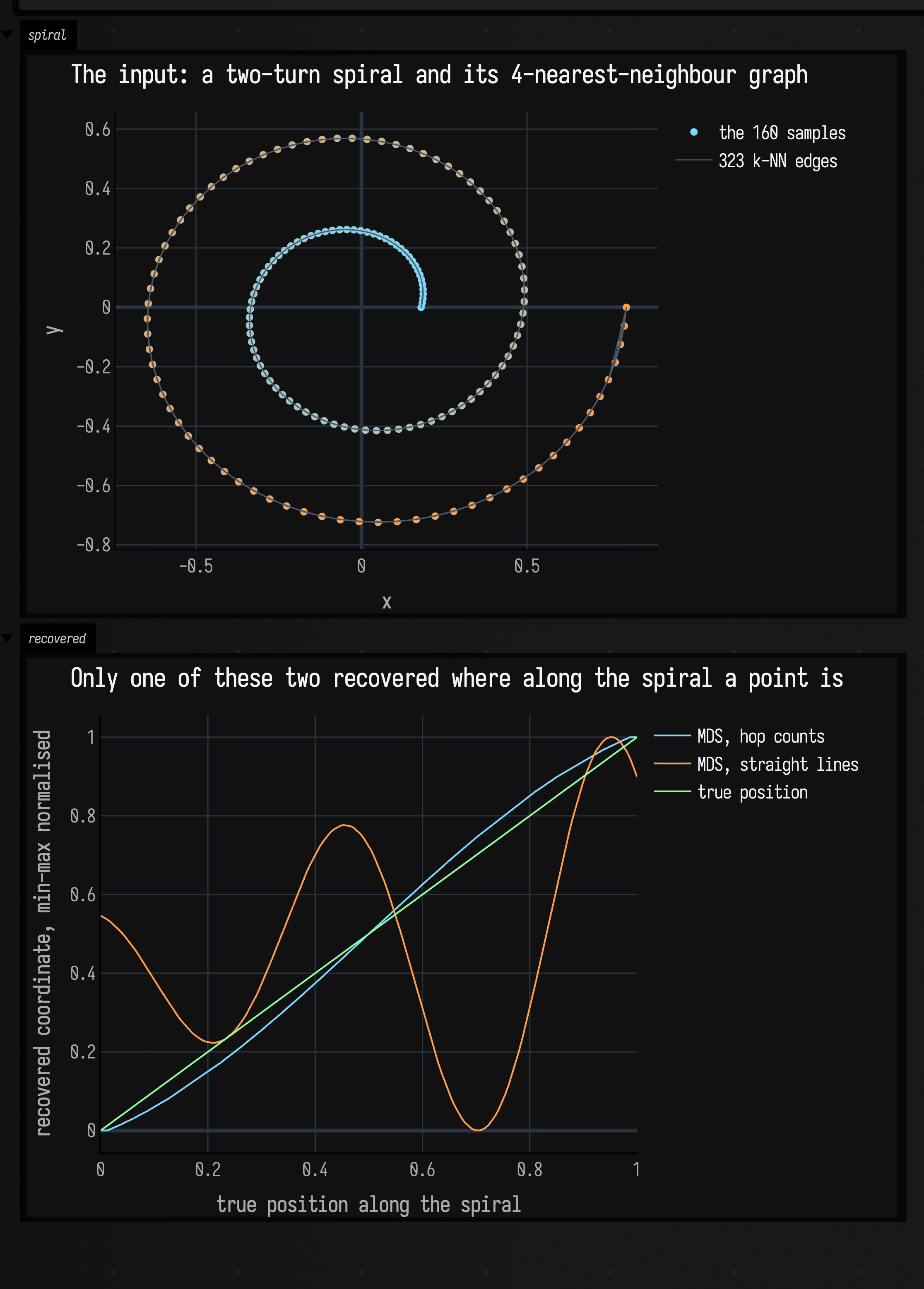
The number under the second figure is 1.0000. MDS on hop counts recovers a coordinate whose rank order along the spiral is exactly the true one, a Spearman rho of 1.0000 with no exceptions in 160 points, while the same MDS on straight-line distances gets 0.2325, because in two dimensions the straight-line fit can only reproduce the spiral, and the spiral's x-coordinate crosses the same value four times. Against a fitted arc length rather than a rank, the graph coordinate is linear at Pearson 0.9852 against 0.3238.
Both fits are the same call with the same options; only the distance matrix differs. Change the matrix and the projection answers a different question.
The thing to check is the graph, and the fence checks it: worst \( \lvert i - j \rvert \) over an edge = 4,
so no edge has jumped between arms. A single shortcut edge would collapse two arms into one and the
rho above would fall off a cliff. Raise k until that happens and you can watch it go.
MDS against t-SNE
The usual advice is that MDS preserves global distances and t-SNE preserves local neighbourhoods. Both are true; what decides whether you can read a number off the picture is how big each distortion is.
Three Gaussian clusters of sixty points each in twelve dimensions, with unit spread and centres placed so that one fact is checkable: cluster 1 is 10 away from cluster 0 and cluster 2 is 40 away. So one true fact about the data is that clusters 0 and 2 are about four times further apart than clusters 0 and 1, and either projection keeps that or it does not.
:::static
import space.kscience.plotly.*
import space.kscience.plotly.models.ScatterMode

val dimensions = 12
val perCluster = 60
val rng = java.util.Random(4)
val centres = [
    DoubleArray(dimensions),
    DoubleArray(dimensions).also { it[0] = 10.0 },
    DoubleArray(dimensions).also { it[1] = 40.0 },
]
val data = ArrayList<DoubleArray>()
val label = ArrayList<Int>()
centres.forEachIndexed { cluster, centre ->
    repeat(perCluster) {
        data += DoubleArray(dimensions) { centre[it] + rng.nextGaussian() }
        label += cluster
    }
}
val vectors = data.toTypedArray()
val n = vectors.size

val mds = smileMds(vectors, dimensions = 2, distance = SmileMdsDistance.EUCLIDEAN, positiveCorrection = false)
val tsne = smileTsne(vectors, dimensions = 2, distance = SmileMdsDistance.EUCLIDEAN, perplexity = 30.0)

// Measurement one: the ratio of two between-cluster distances. Scale-free on purpose, because
// neither projection promises to keep the units, and a ratio is what a reader takes off a picture.
val gap = { coordinates: Array<DoubleArray>, a: Int, b: Int ->
    val centroid = { cluster: Int ->
        val rows = (0 until n).filter { label[it] == cluster }
        DoubleArray(coordinates[0].size) { c -> rows.sumOf { coordinates[it][c] } / rows.size }
    }
    val ca = centroid(a)
    val cb = centroid(b)
    sqrt(ca.indices.sumOf { (ca[it] - cb[it]).let { d -> d * d } })
}
val ratio = { coordinates: Array<DoubleArray> -> gap(coordinates, 0, 2) / gap(coordinates, 0, 1) }

// Measurement two: of each point's ten nearest neighbours in twelve dimensions, how many are still
// among its ten nearest in the plane?
val nearest = { source: Array<DoubleArray>, row: Int, k: Int ->
    (0 until n)
        .filter { it != row }
        .sortedBy { other -> source[row].indices.sumOf { (source[row][it] - source[other][it]).let { d -> d * d } } }
        .take(k)
        .toSet()
}
val recall = { coordinates: Array<DoubleArray>, k: Int ->
    (0 until n).sumOf { row -> nearest(vectors, row, k).intersect(nearest(coordinates, row, k)).size / k.toDouble() } /
        n
}

println(
    "true    0-1 ${gap(vectors, 0, 1).f3}  0-2 ${gap(vectors, 0, 2).f3}  ratio ${ratio(vectors).f4}",
)
println(
    "MDS     0-1 ${gap(mds.coordinates, 0, 1).f3}  0-2 ${gap(mds.coordinates, 0, 2).f3}  ratio ${ratio(mds.coordinates).f4}",
)
println(
    "t-SNE   0-1 ${gap(tsne.coordinates, 0, 1).f3}  0-2 ${gap(tsne.coordinates, 0, 2).f3}  ratio ${ratio(tsne.coordinates).f4}",
)
println(
    "10-nearest-neighbour recall: MDS ${recall(mds.coordinates, 10).f4}, " +
        "t-SNE ${recall(tsne.coordinates, 10).f4}",
)

// Perplexity is the dial between the two, so sweep it rather than describing it.
val sweep =
    [5.0, 30.0, 100.0].map { perplexity ->
        val fit = smileTsne(vectors, dimensions = 2, distance = SmileMdsDistance.EUCLIDEAN, perplexity = perplexity)
        Triple(perplexity, ratio(fit.coordinates), recall(fit.coordinates, 10))
    }
sweep.forEach { (perplexity, gapRatio, knn) ->
    println(
        "t-SNE perplexity ${perplexity.f0}: ratio ${gapRatio.f4}, recall ${knn.f4}",
    )
}

// The seed matters, and it matters in one direction only.
val again = smileTsne(vectors, dimensions = 2, distance = SmileMdsDistance.EUCLIDEAN, perplexity = 30.0)
val other = smileTsne(vectors, dimensions = 2, distance = SmileMdsDistance.EUCLIDEAN, perplexity = 30.0, seed = 7L)
val drift = { a: Array<DoubleArray>, b: Array<DoubleArray> ->
    (0 until n).maxOf { row -> (0..1).maxOf { c -> abs(a[row][c] - b[row][c]) } }
}
println("refit at the default seed: worst coordinate difference ${drift(tsne.coordinates, again.coordinates)}")
println(
    "refit at seed 7: worst coordinate difference ${drift(tsne.coordinates, other.coordinates).f4}, " +
        "cost ${tsne.cost.f4} vs ${other.cost.f4}",
)
:::fold the two planes, side by side
val palette = ["#7ad9ff", "#ff9e4a", "#8fff9a"]
val panel = { coordinates: Array<DoubleArray>, caption: String ->
    Plotly.plot {
            (0..2).forEach { cluster ->
                val rows = (0 until n).filter { label[it] == cluster }
                scatter {
                    name = "cluster $cluster"
                    mode = ScatterMode.markers
                    x.set(rows.map { coordinates[it][0] })
                    y.set(rows.map { coordinates[it][1] })
                    marker {
                        size = 5.0
                        color(palette[cluster])
                    }
                }
            }
            layout {
                title = caption
                xaxis { title = "coordinate 1" }
                yaxis { title = "coordinate 2" }
            }
        }
        .darkMode()
}
display(
    "mds",
    panel(
        mds.coordinates,
        "MDS: centre 0-2 is ${ratio(mds.coordinates).f2}x centre 0-1 (truth: ${ratio(vectors).f2}x)",
    ),
)
display(
    "tsne",
    panel(tsne.coordinates, "t-SNE, perplexity 30: the same ratio reads ${ratio(tsne.coordinates).f2}x"),
)
:::endfold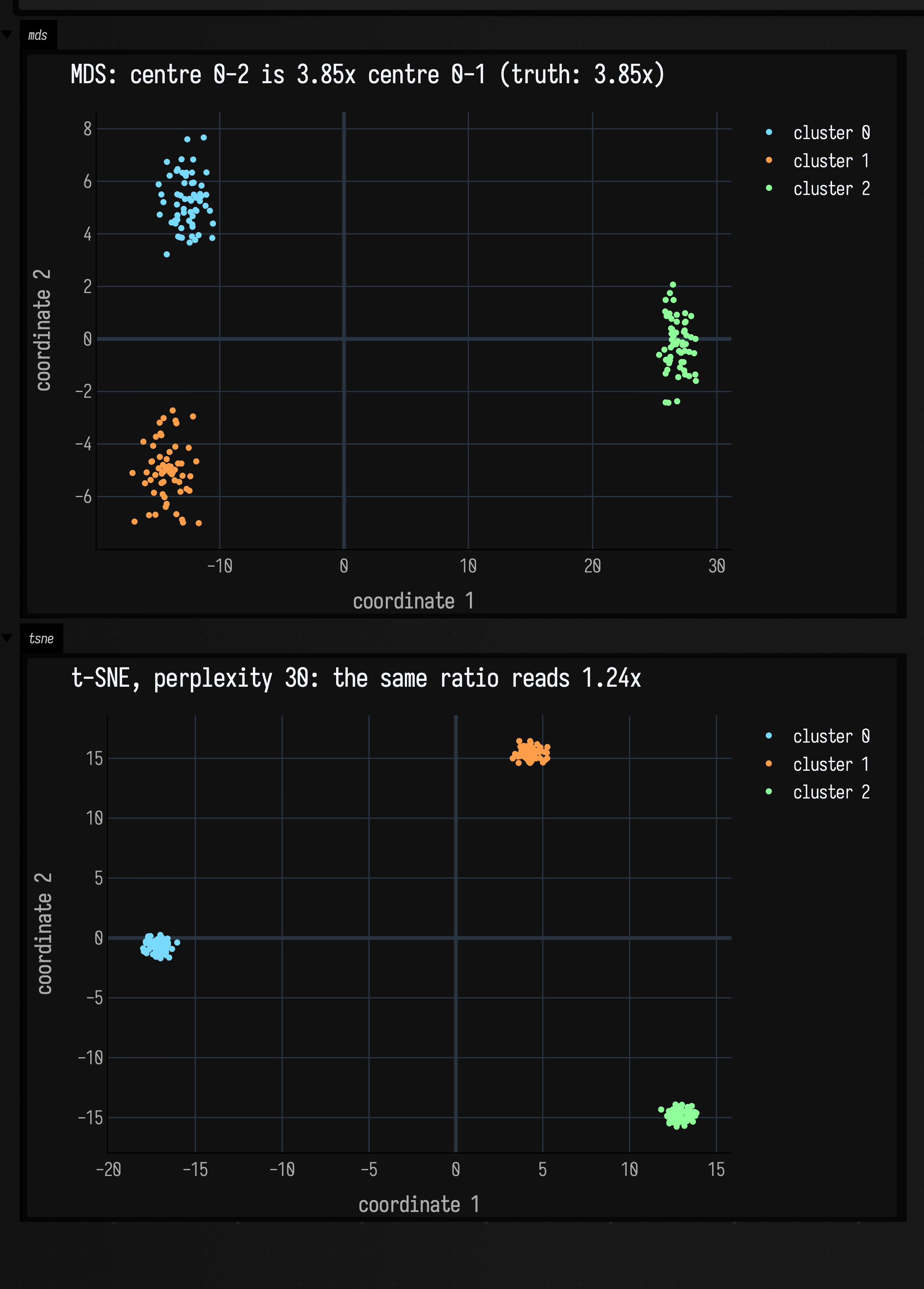
The two panels show the same data and disagree about the most obvious thing in it.
| Embedding | between-centre ratio 0–2 : 0–1 | 10-nearest-neighbour recall |
|---|---|---|
| truth, in twelve dimensions | 3.8485 | 1.0 by definition |
| MDS | 3.8489 | 0.2922 |
| t-SNE, perplexity 30 | 1.2369 | 0.4761 |
MDS gets the global geometry right to four significant figures, 3.8489 against 3.8485, which is not a surprise once you see why: the three centres span a two-dimensional subspace of the twelve, so two components are genuinely enough to hold them. And it pays for that with the worst local structure of anything here: of each point's ten nearest neighbours in twelve dimensions, MDS keeps 2.9.
t-SNE inverts both. It keeps 4.8 of the ten neighbours, 63% more than MDS, and it reports the two clusters that are 3.85 times further apart as 1.24 times further apart. The distance you would read off that picture is wrong by a factor of 3.1. That is why you should never read distances between t-SNE clusters.
Perplexity is the dial between the two behaviours, and the sweep is monotone in both directions at once:
| perplexity | between-centre ratio | 10-NN recall |
|---|---|---|
| 5 | 1.0247 | 0.5067 |
| 30 | 1.2369 | 0.4761 |
| 100 | 3.2761 | 0.2894 |
At perplexity 5 the three clusters come out essentially equidistant, a ratio of 1.02 against a true 3.85, with the best local structure on the page. At 100 the ratio is nearly right at 3.28 and the local recall has fallen below MDS's. So a t-SNE plot cannot be read at all without knowing its perplexity, and the default of 30 sits at the end of that range where global distance means least.
The seed matters as much. Two fits of the same data at the same seed are bit-identical, which is
what makes a live-coded box redraw the same picture when you re-run it. Two fits at different
seeds are not remotely the same picture: the worst coordinate moves by 30.59 while the reported
cost barely moves at all, 0.1709 against 0.1707 — an equally good answer and a completely
different plot. If a t-SNE figure is going into something anyone else will read, the seed belongs in
the caption.
Why same-seed fits are identical
Smile's t-SNE initialiser draws from smile.math.MathEx's process-wide random source, so
smileTsne installs seed and runs the fit inside a lock
(smile_mds.kt:156). The worst coordinate difference between
two same-seed fits above is exactly 0.0.
The lock also means concurrent t-SNE fits queue rather than parallelise. On a long fit that is visible, and it is the price of the guarantee.
positiveCorrection
A cosine distance is not Euclidean. Neither is an edit distance or a hop count. For such a matrix
the double-centred learning matrix has negative eigenvalues, and classical MDS has nothing to take a
square root of. positiveCorrection, on by default, adds a constant to every off-diagonal
dissimilarity, chosen as the largest real eigenvalue of a 2n × 2n system, until the matrix is
positive semi-definite (smile_mds.kt:409).
The word-distance matrix from the first fence is a clean test, because Levenshtein is a metric that obeys the triangle inequality and is still not Euclidean.
:::static
val families = [
    ["compute", "computes", "computed", "computer", "computing"],
    ["render", "renders", "rendered", "renderer", "rendering"],
    ["listen", "listens", "listened", "listener", "listening"],
    ["sample", "samples", "sampled", "sampler", "sampling"],
]
val words = families.flatten()
val wordEditDistance = { a: String, b: String ->
    var previous = IntArray(b.length + 1) { it }
    for (i in 1..a.length) {
        val current = IntArray(b.length + 1)
        current[0] = i
        for (j in 1..b.length) {
            val substitution = previous[j - 1] + if (a[i - 1] == b[j - 1]) 0 else 1
            current[j] = minOf(previous[j] + 1, current[j - 1] + 1, substitution)
        }
        previous = current
    }
    previous[b.length]
}
val distances =
    Array(words.size) { a ->
        DoubleArray(words.size) { b -> wordEditDistance(words[a], words[b]).toDouble() }
    }

// How many dimensions will each setting give you before the spectrum runs out of positive
// eigenvalues? Ask for more and more until the call refuses.
val spectra =
    [false, true].map { correction ->
        var accepted = 0
        var scores = DoubleArray(0)
        var refusal = "never refused"
        for (dimension in 2..18) {
            try {
                val fit = smileMdsDistances(distances, dimensions = dimension, positiveCorrection = correction)
                accepted = dimension
                scores = fit.scores
            } catch (refused: IllegalArgumentException) {
                refusal = refused.message.orEmpty().substringAfter("smileMds: ")
                break
            }
        }
        Triple(correction, accepted, scores) to refusal
    }
spectra.forEach { (result, refusal) ->
    val (correction, accepted, scores) = result
    println("positiveCorrection = $correction: largest usable dimensions = $accepted")
    println("  spectrum ${scores.joinToString { it.f2 }}")
    println("  $refusal")
}

// And what it costs in the plane, which is the part that is easy to guess wrong.
[false, true].forEach { correction ->
    val fit = smileMdsDistances(distances, dimensions = 2, positiveCorrection = correction)
    println(
        "two dimensions, positiveCorrection = $correction: " +
            "r = ${fit.distanceCorrelation.f4}, stress-1 = ${fit.stress1.f4}",
    )
}
:::fold the two spectra
showSignals(
    "positiveCorrection = false" to spectra[0].first.third.toList(),
    "positiveCorrection = true" to spectra[1].first.third.toList(),
    channel = "spectra",
    title = "Eigenvalue spectrum of a Levenshtein matrix, corrected and not",
    xTitle = "component",
    yTitle = "eigenvalue",
)
:::endfold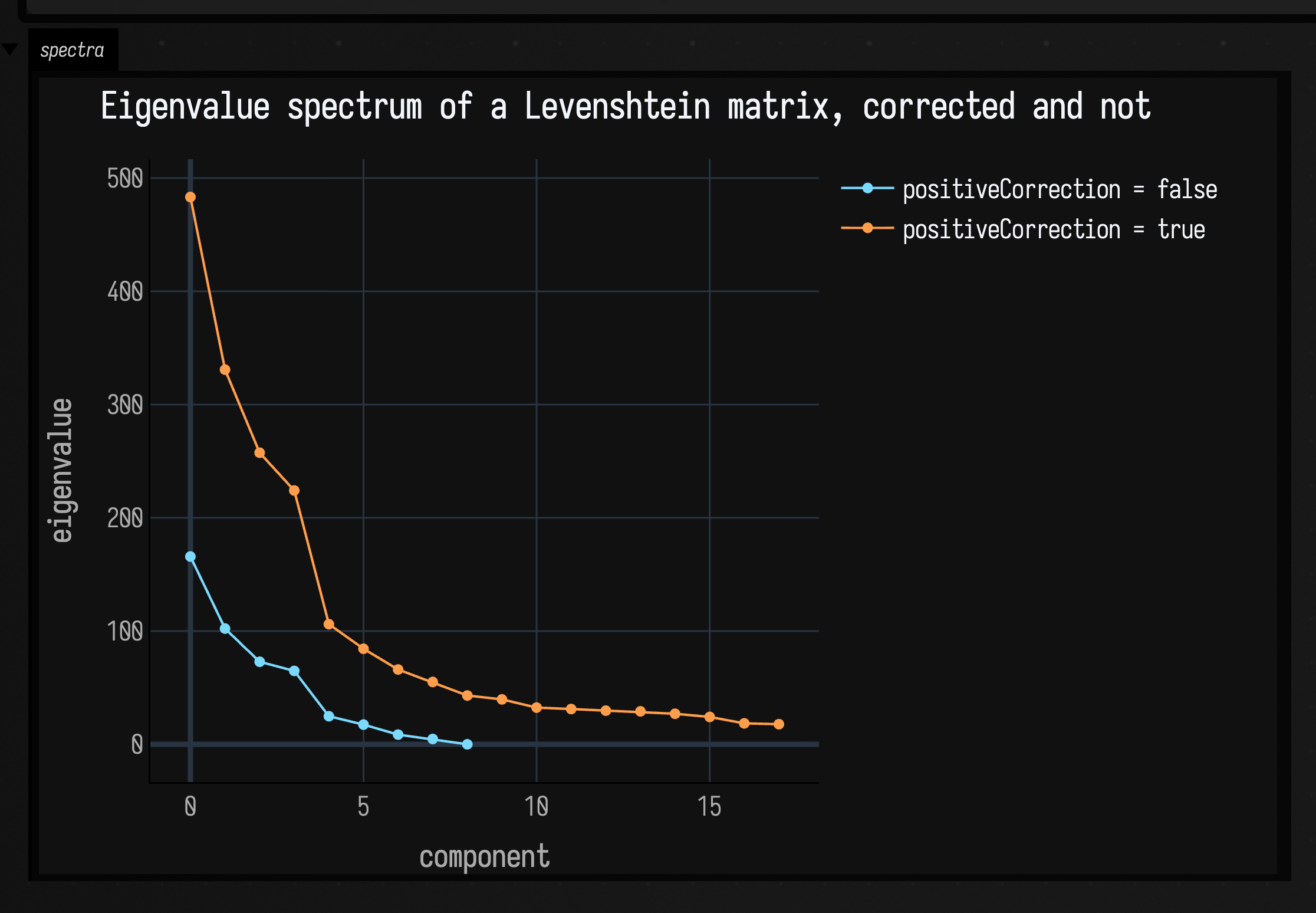
Uncorrected, this matrix gives you 9 dimensions and no more. The spectrum runs 165.81, 102.20, 72.87, 64.80, 24.78, 17.39, 8.54, 4.70, then a ninth component at machine zero, and the tenth is genuinely negative at −1.03, at which point the call refuses, because there is no real square root of a negative eigenvalue. Corrected, all 18 requestable dimensions are comfortably positive, the smallest of them 17.75.
So the flag gives you more dimensions. It does not make the fit more accurate: in two dimensions the uncorrected fit is
fractionally the better of the two, at r 0.8533 and stress 0.2626 against 0.8475 and 0.2780 with the
correction on. The additive constant inflates every distance by the same amount, which flattens the
relative differences the projection is trying to reproduce. So if you only ever want two or three
components out of a non-Euclidean matrix, positiveCorrection = false is sometimes slightly
better; the default is true because "the call throws for reasons about the
tenth eigenvalue" is a worse first experience than losing 0.015 of a correlation.
Sharp edges
- The proximity matrix is \( n^2 \) doubles, and Smile allocates more on top. 7.6 MiB at n = 1000,
191 MiB at 5000, 3.0 GiB at 20 000, 19 GiB at 50 000. A long trajectory has to be sampled before
it is projected.
smileMdsbuilds the matrix itself (smile_mds.kt:111), so the cost applies even when you never see it. - MDS axes have arbitrary sign and arbitrary rotation. They are eigenvectors; nothing pins the direction. The spiral fence flips the sign to agree with the known parameter before comparing, and any code that compares two fits has to do something equivalent.
- A rank-deficient fit is fine; a negative eigenvalue is not. Asking for as many components as
the data has structure gives a column of zeros, which is correct. Asking for more than an
uncorrected non-Euclidean matrix can support raises
IllegalArgumentException(smile_mds.kt:440). - t-SNE needs at least four rows and a perplexity below the row count, and its axes carry no meaning at all: not units, not order, not orientation. Only the neighbourhoods do.
Choosing between MDS and t-SNE
If the quantity you want to read off the picture is a distance, as in this pair being twice as far
apart as that pair, use MDS, and report a stress figure alongside it so the reader knows what two dimensions
cost. If the quantity you want is membership, as in these things belonging together and that one
not, use t-SNE, quote the perplexity and the seed, and do not let anyone measure between the clumps. If
your things are vectors and cosine or Euclidean is the right distance, smileMds and smileTsne
build the matrix for you; if the distance is something only you can compute, whether an edit distance, a
transport cost, a hop count or a diff size, smileMdsDistances and smileTsneDistances are the
entry points, and the two worked examples above are both of that kind. Above a few thousand things,
sample first: everything here is quadratic in memory before it is anything else.
For the audio-specific wrappers over these same four functions, see speech-reactive learned spaces and short-time spectral spaces; for the graph constructions the second fence borrows, Neighbors & graphs; and for the dependence coefficients the fences use to check themselves, Statistics & dependence.
The public declarations used on this page are listed, with their KDoc, in the codebase reference: Data and Math.