Points into structure — Voronoi, Apollonius, contours and clusters
Given a set of points, much of what you might do with them comes down to one question: which part of the plane belongs to which point, and where are the boundaries between them?
Field has four ways to answer it, all in Field's standard library, and this page works through each:
- Delaunay triangulation and its Voronoi dual: the classical answer, exact, built on JTS.
- Apollonius (multiplicatively weighted Voronoi): the same question with the points given sizes, where the boundaries become circular arcs.
- Marching squares: the boundaries of a field rather than of a point set, extracted as drawable geometry.
- Clustering: grouping the points instead of dividing the plane.
Where the family lives
The filenames do not match their contents well, so here is what lives where:
| what you want | where it is | notes |
|---|---|---|
| 2D Delaunay, 2D Voronoi, 2D convex hull | graph_connectivity.kt |
vec2DelaunayGraph, vec2DelaunayTriangles, vec2VoronoiDiagram, vec2VoronoiDualGraph, vec2ConvexHull. JTS-backed and exact. See also Neighbors & Graphs |
| 2D weighted (Apollonius) Voronoi | dirichlet.kt |
CircularDirichlet. Pure Kotlin. Not Poisson-disc sampling, despite the name |
| 3D Voronoi, 3D weighted Voronoi | voronoi.kt |
voronoi3d, CircularDirichlet3d. voronoi.kt has no 2D anything and no Delaunay at all |
marching squares → polylines and FLines |
contours.kt |
generateIsoContours, generateSmoothIsoContours, pointEdgeScalarField2D |
| clustering | clustering.kt |
agglomerative (7 linkages), k-medoids, k-medians. There is no k-means in Field — see below for why |
any of the above → FLine |
spatial_field.kt |
toFLine/toFLines per result type, plus showPlane / showPlaneGrid |
The last row makes the rest drawable. Every partitioner above answers with structure (vertex
rings, circular arcs, triangle index triples, integer labels) rather than with geometry, and
spatial_field.kt converts one to the other. It is the plane counterpart of
mesh_field.kt in Meshes & 3D Geometry.
Delaunay, and the Voronoi dual
Start with the classical pair, because they are the same object seen twice. Given n sites:
- the Voronoi diagram cuts the plane into one cell per site, every point in a cell being nearer to that site than to any other;
- the Delaunay triangulation joins two sites exactly when their cells share an edge.
Each determines the other, which is why vec2VoronoiDualGraph(points) simply returns
vec2DelaunayGraph(points).
The example below triangulates a jittered grid of 54 sites, builds their Voronoi cells and convex hull, and draws all three in a grid of panels whose captions report the counts.
:::static
// A jittered lattice: structured enough that you can see the answer is right, irregular enough
// that the triangulation has something to decide.
val rng = java.util.Random(17)
val sites =
    (0 until 54).map { i ->
        vec((i % 9) * 44.0 + rng.nextDouble() * 22.0, (i / 9) * 44.0 + rng.nextDouble() * 22.0)
    }

val delaunay = vec2DelaunayGraph(sites) // a PointGraph: index pairs
val triangles = vec2DelaunayTriangles(sites) // List<Triple<Int, Int, Int>>: the faces
val voronoi = vec2VoronoiDiagram(sites) // one VoronoiCell per site, each a vertex ring
val hull = vec2ConvexHull(sites) // ConvexHull2D: hullPoints + hullIndices

/*
Euler's formula pins both counts exactly, so this is an assertion and not an observation:
a triangulation of n points with h of them on the convex hull has 2n - 2 - h triangles and
3n - 3 - h edges. Nothing else is a valid triangulation.
*/
val n = sites.size
val h = hull.hullIndices.size
val trianglesExpected = 2 * n - 2 - h
val edgesExpected = 3 * n - 3 - h

/*
The cells of the h hull sites are *unbounded*, and JTS returns them clipped to a generous
envelope rather than to anything you asked for: measured here, the cell vertices span
-423..799 in x while the sites only span 7..369. Fit a figure to that and the diagram
collapses into a speck. So pin the window explicitly and let showPlaneGrid cut the rest.
*/
val window = Rect(
    sites.minOf { it.x.toDouble() } - 18.0,
    sites.minOf { it.y.toDouble() } - 18.0,
    sites.maxOf { it.x.toDouble() } - sites.minOf { it.x.toDouble() } + 36.0,
    sites.maxOf { it.y.toDouble() } - sites.minOf { it.y.toDouble() } + 36.0,
)
val bounded =
    voronoi.cells.count { c ->
        c.vertices.size >= 3 &&
            c.vertices.all {
                it.x >= window.x && it.x <= window.x + window.w && it.y >= window.y && it.y <= window.y + window.h
            }
    }
:::fold draw the three panels
val cloud = pointCloudFLine(sites, color = vec(1.0, 1.0, 1.0, 0.9), pointSize = 1.1)
val frame = window.toFLine(color = vec(0.35, 0.44, 0.56, 0.55), thickness = 1.0)
val hullLine = polylineFrom(hull.hullPoints, 0, closed = true).also {
    it.color = vec(1.0, 0.78, 0.36, 0.85)
    it.thickness = 2.0
}

showPlaneGrid(
    "vec2DelaunayTriangles — the faces\n${triangles.size} triangles, expected 2n-2-h = $trianglesExpected" to
        [frame, delaunayTrianglesToFLine(sites, triangles, color = vec(0.55, 0.70, 0.88, 0.6)), cloud],
    "vec2VoronoiDiagram — the dual\n${voronoi.cells.size} cells for $n sites, $bounded of them wholly inside this window" to
        listOf(frame, *voronoi.toFLines(palette = okhslSet(n, 0.7, 0.62, 0.9f), thickness = 1.2).toTypedArray(), cloud),
    "both, plus vec2ConvexHull\n${delaunay.edges.size} Delaunay edges, expected 3n-3-h = $edgesExpected; $h sites on the hull" to
        listOf(
            frame,
            delaunay.toFLine(sites, color = vec(0.45, 0.58, 0.75, 0.6), thickness = 1.0),
            *voronoi.toFLines(color = vec(0.62, 0.92, 1.0, 0.62), thickness = 1.1).toTypedArray(),
            hullLine,
            cloud,
        ),
    columns = 2,
    cellWidth = 430,
    cellHeight = 280,
    window = window,
)
:::endfold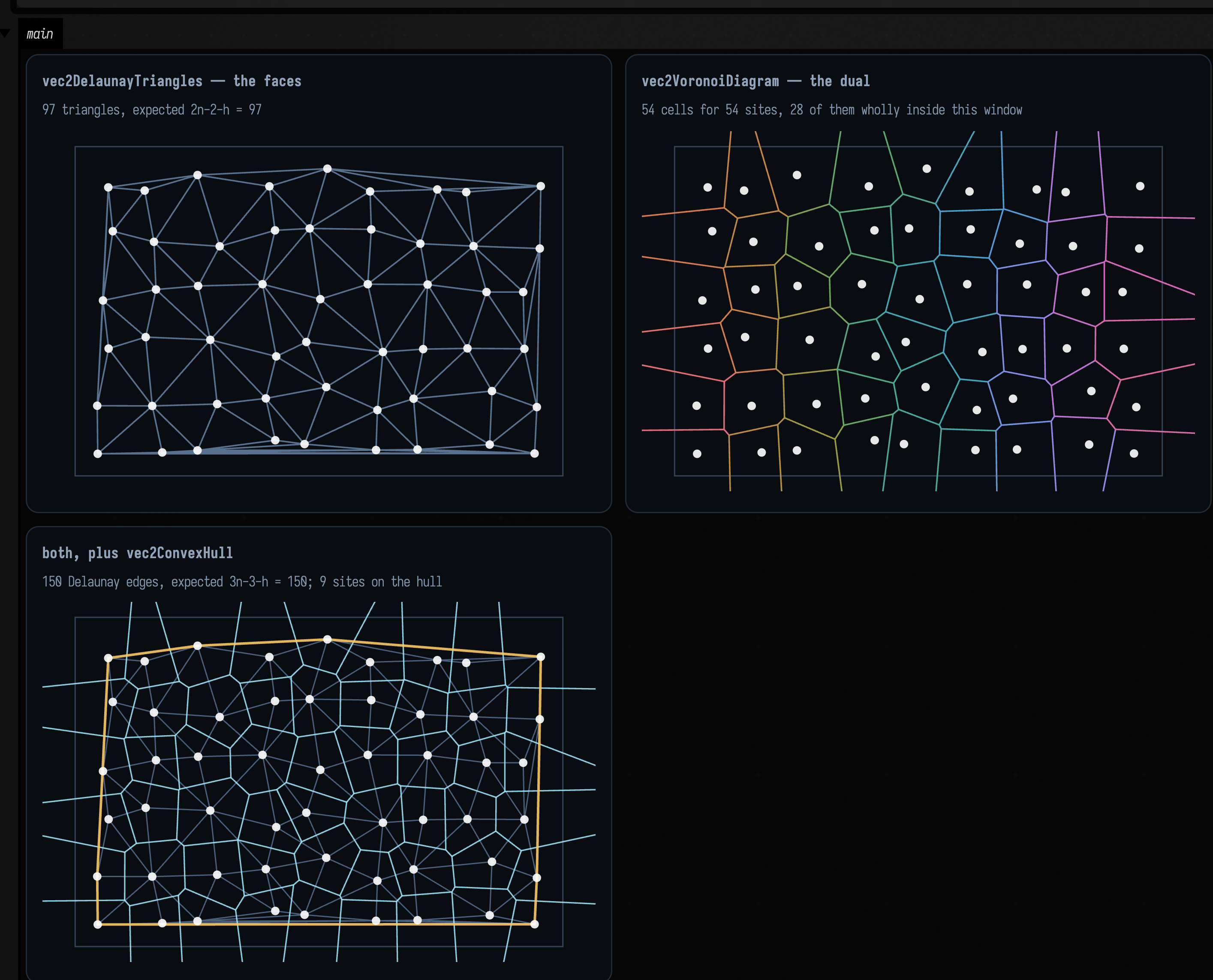
Read the captions. The triangulation reports 97 triangles against Euler's 2·54 − 2 − 9 = 97, and 150 edges against 3·54 − 3 − 9 = 150, with 9 sites on the hull. Every triangulation of a given point set has exactly that many faces and edges, so the two numbers check the structure of the result. The third panel is the duality itself: every Delaunay edge crosses exactly one Voronoi edge, and crosses it at right angles, because a Voronoi edge is the perpendicular bisector of the two sites it separates. Every Voronoi vertex sits at the circumcentre of one Delaunay triangle.
Two properties to know before you build on this:
- The cells on the hull are unbounded, and JTS clips them to a generous bounding envelope
rather than returning infinite rings. Here the cell vertices span −423 … 799 in x while
the sites only span 7 … 369, so a figure fitted to the cells shrinks the diagram to a speck
in the middle. That is why the example sets its own
windowand draws it:showPlaneGridclips to the frame, and the caption reports how many cells are wholly inside it (28 of 54). A boundary cell's vertex ring is real geometry, but its area is an artefact of the clip, not of the sites. VoronoiCell.verticesis the ring, not a polygon object. Draw it withpolylineFrom(cell.vertices, closed = true), or useVoronoiDiagram.toFLines(), which does it for you and drops the empty cells JTS returns for a duplicated site.
vec2DelaunayGraph is one of a family (Gabriel, Urquhart, relative-neighbourhood, β-skeleton, kNN,
minimum spanning tree) that all return a PointGraph, and PointGraph.toFLine(points) draws any
of them. Neighbors & Graphs compares them.
When the bisector is a circle
Now give each site a weight and ask the same question. CircularDirichlet minimises
score_i(x) = |x - p_i|² / w_i²which is the multiplicatively weighted or Apollonius diagram: a site with twice the weight claims points twice as far away. This is the model you want whenever the sites are not interchangeable: cities of different populations, cell nuclei of different sizes, sound sources of different loudness, brush marks of different pressure.
The consequence is geometric. Setting score_i(x) = score_j(x) for two sites
gives, after clearing denominators, the equation of a circle, the Apollonius circle of the two
points in the ratio w_i : w_j. It degenerates to a straight line only when w_i = w_j. So a
weighted Voronoi cell is not a polygon: its boundary is made of circular arcs, and the API hands
you those arcs rather than flattening them:
val diagram = CircularDirichlet.build(sites) // sites are Vec3 of (x, y, weight)
val cell = diagram[0] // a CellBoundary
cell.pieces // ArcPiece | LinePiece, angularly sorted
piece.support // SupportCircle(center, radius) or SupportLine
piece.samplePoint() // a point known to be on this boundary
piece.toPolyline(maxChordError = 0.02f, clip = box)
The figure keeps five sites in the same places and changes only their weights: all equal, mixed, and one site much heavier than the rest.
:::static
// Sites are (x, y, weight). Same five positions in all three panels; only the weights change.
val positions = [
    vec(0.0, 0.0),
    vec(2.2, 0.3),
    vec(0.9, 2.0),
    vec(-1.4, 1.1),
    vec(1.1, -1.6),
]
val clip = CircularDirichlet.Aabb(vec(-3.4, -3.4), vec(4.6, 4.6))

fun diagramOf(weights: List<Double>) =
    CircularDirichlet.build(positions.mapIndexed { i, p -> vec(p.x, p.y, weights[i]) })

val equal = diagramOf(List(5) { 1.0 })
val mixed = diagramOf([1.0, 1.35, 0.8, 1.1, 1.6])
val swallowed = diagramOf([1.0, 2.6, 1.0, 1.0, 1.0])

// With equal weights every bisector degenerates to a straight line: a line only when the weights
// match. These two counts go into the captions below.
fun arcCount(d: CircularDirichlet.Diagram) = d.cells.sumOf { c -> c.pieces.count { it is CircularDirichlet.ArcPiece } }
fun lineCount(d: CircularDirichlet.Diagram) =
    d.cells.sumOf { c -> c.pieces.count { it is CircularDirichlet.LinePiece } }

// A full-sweep arc is a *complete circle*: that cell is a disc, entirely enclosed by one neighbour.
fun fullCircles(d: CircularDirichlet.Diagram) =
    d.cells.sumOf { c ->
        c.pieces.count { it is CircularDirichlet.ArcPiece && it.sweepAngle > 6.283 }
    }
// …and a cell bounded by exactly one full circle is a cell that has been entirely enclosed.
fun enclosedCells(d: CircularDirichlet.Diagram) =
    d.cells.count { c ->
        c.pieces.size == 1 && (c.pieces[0] as? CircularDirichlet.ArcPiece)?.let { it.sweepAngle > 6.283 } == true
    }
:::fold draw the three diagrams
val palette = okhslSet(5, saturation = 0.8, lightness = 0.66)
val cloud = pointCloudFLine(positions, color = vec(1.0, 1.0, 1.0, 0.95), pointSize = 1.6)

fun panel(d: CircularDirichlet.Diagram) =
    d.toFLines(clip = clip, maxChordError = 0.01f, palette = palette, thickness = 1.6) + cloud

showPlaneGrid(
    "equal weights — a plain Voronoi diagram\n${lineCount(equal)} straight bisectors, ${arcCount(equal)} arcs" to
        panel(equal),
    "weights 1.0 / 1.35 / 0.8 / 1.1 / 1.6\n${arcCount(mixed)} arcs, ${lineCount(mixed)} straight" to panel(mixed),
    "one site at weight 2.6\n${fullCircles(swallowed)} pieces are COMPLETE circles; ${enclosedCells(swallowed)} cells wholly enclosed" to
        panel(swallowed),
    columns = 2,
    cellWidth = 430,
    cellHeight = 280,
)
:::endfold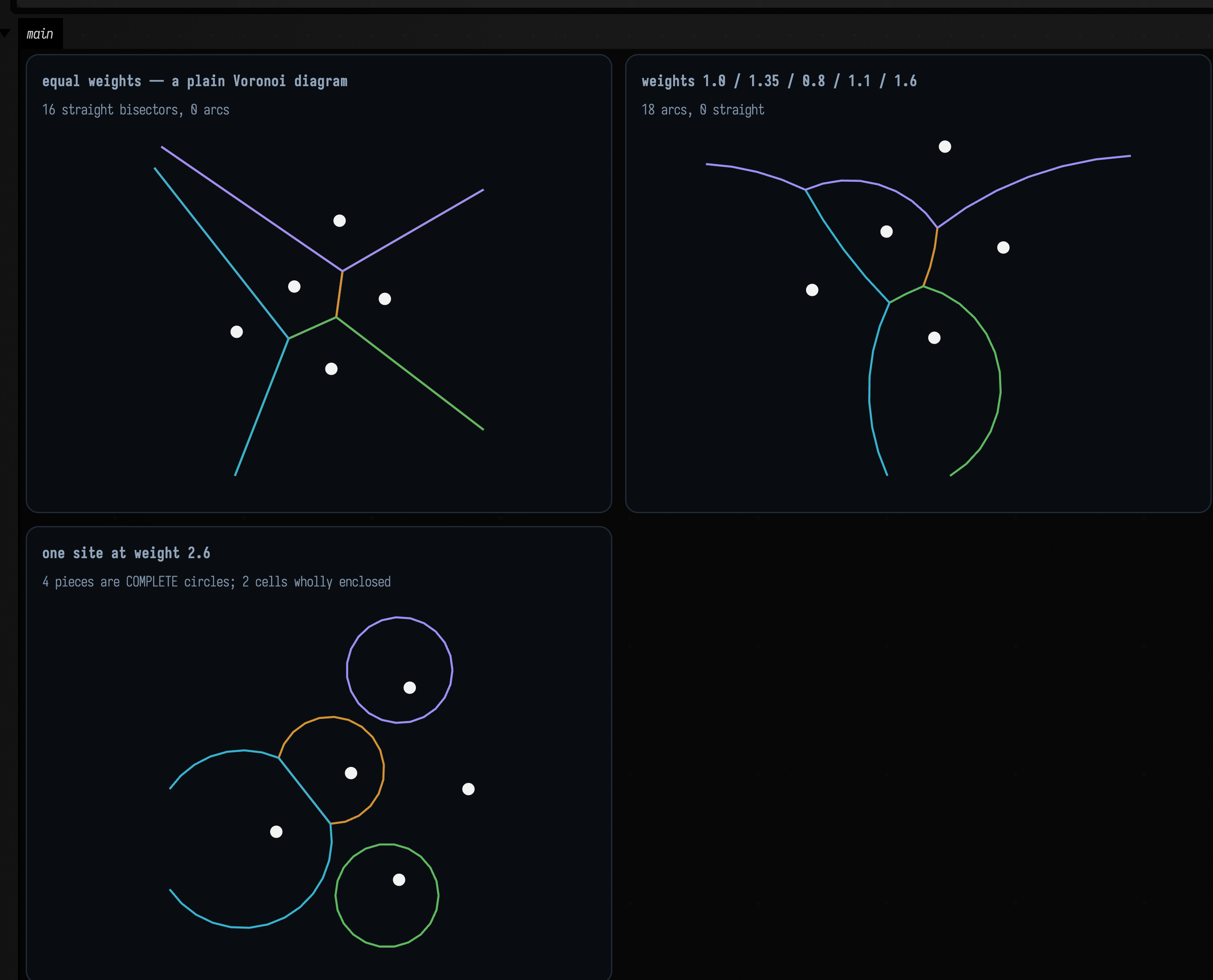
In the middle panel those are arcs: they bulge away from the heavier site, and no polygon construction will produce them. At equal weights the diagram reports 16 straight bisectors and 0 arcs, and at mixed weights 18 arcs and 0 straight. The type of every piece is decided by an exact equality of weights, so the counts are all-or-nothing. Neither count is 20, the number of ordered site pairs: a bisector only becomes a boundary piece of a cell where it is actually the nearest tie, and with five sites several of the twenty pairs never appear.
The third panel shows a cell that is not a ring at all. At weight 2.6 the heavy site does more than take a larger share: two of its light neighbours end up entirely enclosed, and their cells are complete discs bounded by a single full-sweep arc. The heavy site's own cell is then the region outside those two discs, which is why the diagram reports four full-circle pieces, two belonging to the enclosed cells and two to the cell enclosing them. It is a cell with holes, not a polygon, and not even simply connected.
That is why CellBoundary.toFLines(...) returns one FLine per piece rather than one per cell.
Joining them into a single path would misrepresent the topology. The supporting circle has a closed
form: for two sites at p_i, p_j with weight ratio k = w_j/w_i, the Apollonius circle is
centred at \( (k^2 p_i - p_j) / (k^2 - 1) \), which is what arc.support.center returns.
Sweeping one site's weight
Three still panels cannot show a bisector turning into a circle, because that happens between them. Here is the same construction with one number swept: site 1's weight, from 1.0 up to 2.7 and back over eight seconds.
Watch three things. First, only the edges that touch site 1 bow. A bisector between two sites of
equal weight stays exactly straight however heavy their neighbour gets, which is why the caption
reports both counts and why they trade against each other as the weight climbs (8 arcs / 10
straight at weight 1.12, 12 arcs / 6 straight by 2.02), and every arc bulges away from the
heavy site.
Second, those counts do not drift; they jump. The bulge grows until two of the light neighbours'
cells pinch shut into complete discs (enclosed goes from 0 to 2 somewhere between weight 2.02 and
2.45), and the total piece count falls when that happens, because a swallowed cell needs one
full-sweep circle where it used to need several arcs and a line. The topology of the diagram
changes along with its shape.
Third, on the way back down the discs re-open and the arcs flatten, and at exactly 1.0 the whole diagram snaps back to straight lines. The type of every boundary piece is decided by an exact equality of weights, so the piece counts jump there while the picture around them moves smoothly.
The sweep below is an animate { } reading AnimationClock, described in
Frames and the animation loop. Because it follows the clock rather than
frameNumber, the sweep takes eight seconds however fast frames are drawn.
:::static
:::fold the same five sites, a fixed window, the palette, and the clock
val positions = [
    vec(0.0, 0.0),
    vec(2.2, 0.3),
    vec(0.9, 2.0),
    vec(-1.4, 1.1),
    vec(1.1, -1.6),
]
val clip = CircularDirichlet.Aabb(vec(-3.4, -3.4), vec(4.6, 4.6))
/*
A FIXED window, not the default fit-to-contents. Left to fit each frame's own bounds the picture
would rescale as the arcs swell, and the sweep would appear to stand still — the same trap that
makes an auto-ranging heatmap of a WFC collapse look like it is going nowhere.
*/
val window = Rect(-3.4, -3.4, 8.0, 8.0)
val palette = okhslSet(5, saturation = 0.8, lightness = 0.66)
val cloud = pointCloudFLine(positions, color = vec(1.0, 1.0, 1.0, 0.95), pointSize = 1.6)
val heavy = 1 // the site whose weight is swept; the other four stay at 1.0
// The recorder makes AnimationClock exactly frameIndex / fps, so matching this to the fence's
// duration produces one complete, repeatable there-and-back sweep.
val sweepSeconds = 8.0
val started = AnimationClock.nowSeconds()

:::endfold

/*
The line that turns elapsed time into the swept parameter — the one line worth reading, and the one
you would change. A triangle ramp rather than a saw, so the clip runs out to 2.7 and back to 1.0
and loops with no jump at the seam.
*/
fun weightAt(elapsed: Double): Double {
    val phase = (elapsed / sweepSeconds) % 1.0
    return 1.0 + 1.7 * (1.0 - abs(1.0 - 2.0 * phase)) // 1.0 -> 2.7 -> 1.0
}

animate {
    val w = weightAt(AnimationClock.nowSeconds() - started)
    val diagram = CircularDirichlet.build(
        positions.mapIndexed { i, p -> vec(p.x, p.y, if (i == heavy) w else 1.0) },
    )
    val arcs = diagram.cells.sumOf { c -> c.pieces.count { it is CircularDirichlet.ArcPiece } }
    val straight = diagram.cells.sumOf { c -> c.pieces.count { it is CircularDirichlet.LinePiece } }
    // A cell bounded by one full-sweep arc is a cell that has been entirely swallowed.
    val enclosed =
        diagram.cells.count { c ->
            c.pieces.size == 1 && (c.pieces[0] as? CircularDirichlet.ArcPiece)?.let { it.sweepAngle > 6.283 } == true
        }
    showPlane(
        // 0.005 rather than the stills' 0.01: a swallowed cell is a whole circle at this scale, and a
        // coarser chord error makes it visibly a dodecagon.
        diagram.toFLines(clip = clip, maxChordError = 0.005f, palette = palette, thickness = 1.6) + cloud,
        title = "site 1 weight %.2f".format(w),
        caption = "$arcs arcs, $straight straight, enclosed $enclosed",
        width = 660,
        height = 660,
        window = window,
    )
}
Three things to know about the implementation:
- It is aimed at modest site counts. The construction is triple-nested over the sites: every bisector is intersected against every other, and each candidate piece is kept only if a midpoint sample really is on the cell boundary. Use it for dozens of sites, not thousands.
- Unbounded pieces need a clip.
LinePiece.toPolylinethrows without anAabb, because a line running to infinity cannot be flattened. Clipping an arc can also cut it into several runs, which is whyArcPiece.toPolylinesexists and returns a list. - All weights must be strictly positive.
buildrequires it.
There is a 3D counterpart, CircularDirichlet3d in voronoi.kt, where the bisector becomes a
sphere and a cell's boundary is made of SpherePatch3/PlanePatch3. It is explicitly
approximate: it extracts patches by clipping a sampled surface mesh with the weighted score
predicate, and its KDoc says it "prefers stable, wound boundary loops over exact symbolic patch
topology". The exact 3D construction is the unweighted one, below.
Contours of a field
The other kind of boundary is a level set. contours.kt samples a ScalarField2D (a plain
(Double, Double) -> Double) on a grid with marching squares and stitches the crossings into
polylines.
A Voronoi diagram is itself a level set: the set of ties in \( \operatorname{argmin}_i \lvert x - p_i \rvert \). Marching squares finds the level sets of any scalar you like, so you can get a soft, rounded Voronoi by contouring a difference of distances, and an exact one by triangulating. The example below does the first, then uses the same machinery to outline a stroke.
:::static
// Six sites; the field is "how much nearer is the closest site than the second closest", which is
// zero exactly on the Voronoi seams and grows into the middle of each cell.
val sites = [
    vec(-1.6, -0.9),
    vec(1.4, -1.2),
    vec(2.0, 1.1),
    vec(-0.2, 1.7),
    vec(-2.1, 0.9),
    vec(0.4, -0.1),
]
val gap: ScalarField2D = { x, y ->
    val d = sites.map { s -> kotlin.math.hypot(x - s.x, y - s.y) }.sorted()
    d[1] - d[0]
}

/*
This field is NON-NEGATIVE: it touches zero exactly on the seams and is positive everywhere else.
Marching squares finds *sign changes*, so iso = 0.0 finds no contours, which is
correct. A small positive level instead traces each cell shrunk inwards by that margin,
and raising it shrinks them further. That is the useful knob.
*/
val levels = [0.05, 0.35, 0.8, 1.4]
val byLevel = levels.map { iso -> iso to generateIsoContours(gap, -3.4, 3.4, -2.9, 2.9, 120, 120, iso) }
val atZero = generateIsoContours(gap, -3.4, 3.4, -2.9, 2.9, 120, 120, 0.0)

// A completely different use of the same machinery: pointEdgeScalarField2D turns an FLine into a
// signed field whose zero set is a tube around it, so contouring at 0.0 outlines a stroke.
val stroke = fline {
    moveTo(-2.4, 1.2)
    cubicTo(-1.0, -2.2, 1.2, 2.4, 2.6, -1.0)
}
val outline = generateSmoothIsoContours(stroke, radius = 0.55, spatialStep = 0.05)
val fat = generateSmoothIsoContours(stroke, radius = 0.55, spatialStep = 0.05, iso = -0.28)
:::fold draw the levels and the tube
fun contourLines(contours: List<List<Vec2>>, color: Vec4, thickness: Double) =
    contours
        .filter { it.size >= 2 }
        .map { c ->
            polylineFrom(c, 0, closed = isoContourClosed(c, -3.4, 3.4, -2.9, 2.9, boundaryEpsilon = 0.05)).also {
                it.color = color
                it.thickness = thickness
            }
        }

val siteDots = pointCloudFLine(sites, color = vec(1.0, 1.0, 1.0, 0.9), pointSize = 1.4)
val ramp = okhslSet(levels.size, saturation = 0.82, lightness = 0.66, startHue = 0.55f)

val stacked =
    byLevel.flatMapIndexed { i, (_, contours) ->
        contourLines(contours, ramp[i], 1.5 - i * 0.15)
    } + siteDots

showPlaneGrid(
    "iso 0.05 — the cells, minus a hairline\n${byLevel[0].second.size} contours, ${byLevel[0].second.sumOf { it.size }} points; at iso 0.0 exactly: ${atZero.size}" to
        (contourLines(byLevel[0].second, vec(0.62, 0.9, 1.0, 0.85), 1.6) + siteDots),
    "iso 0.05 / 0.35 / 0.8 / 1.4 together\ncells shrinking inwards: ${byLevel.map { it.second.size }.joinToString("/")} contours" to
        stacked,
    "generateSmoothIsoContours on an FLine\ntube radius 0.55 and 0.83, ${outline.size} + ${fat.size} outlines" to
        listOf(
            stroke.also {
                it.color = vec(1.0, 1.0, 1.0, 0.30)
                it.thickness = 1.0
            },
            *fat.map {
                    it.also { f ->
                        f.color = vec(0.98, 0.55, 0.42, 0.55)
                        f.thickness = 1.3
                    }
                }
                .toTypedArray(),
            *outline
                .map {
                    it.also { f ->
                        f.color = vec(1.0, 0.82, 0.42, 0.95)
                        f.thickness = 1.6
                    }
                }
                .toTypedArray(),
        ),
    columns = 2,
    cellWidth = 430,
    cellHeight = 280,
)
:::endfold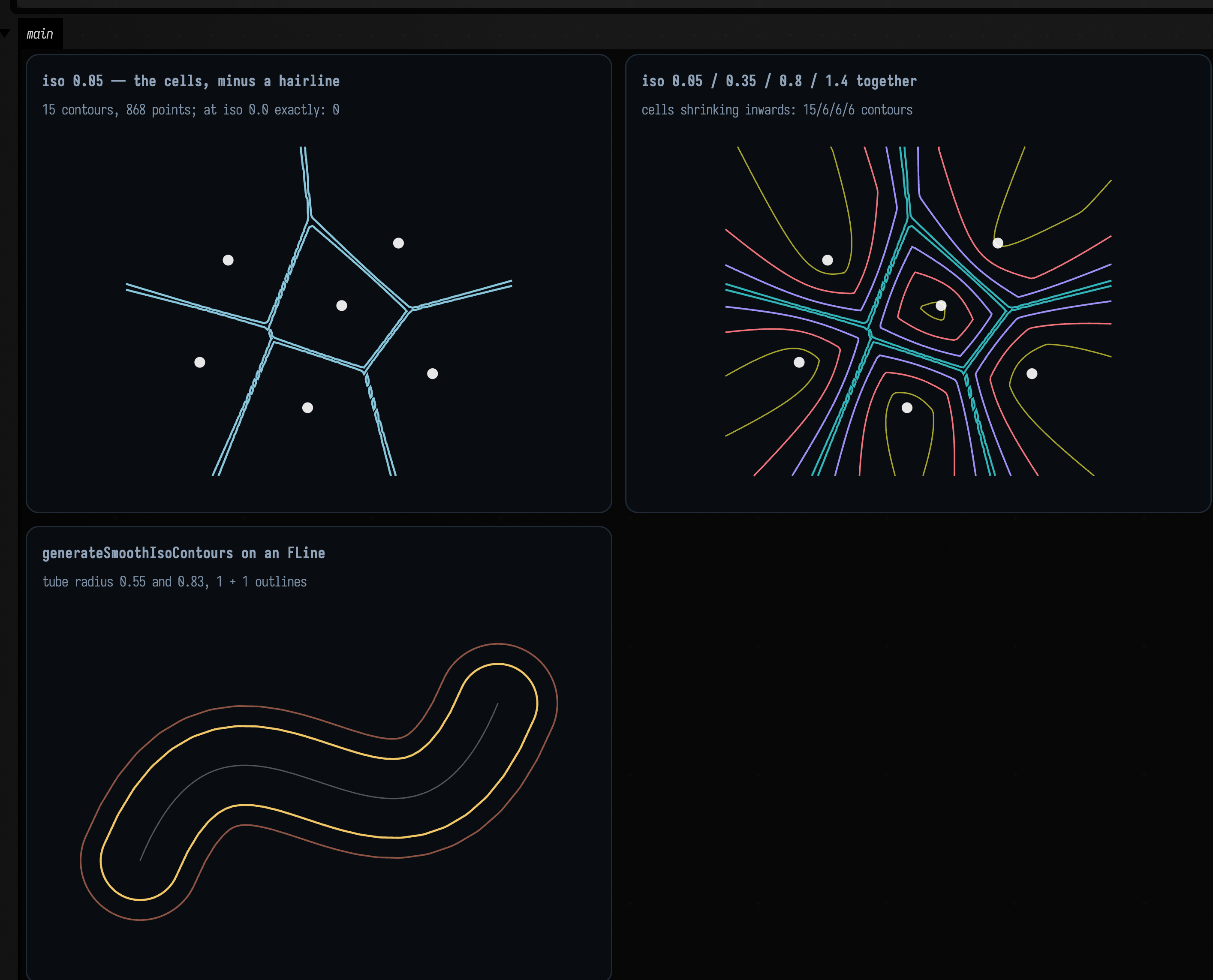
The left panel contours \( d_2 - d_1 \) at a small positive level, which recovers the Voronoi diagram of
the six sites (15 contours, 868 points) by a different algorithm from the Delaunay figure above.
Contour the same field at exactly zero and you get 0 contours, which is correct. Marching
squares locates sign changes, and \( d_2 - d_1 \) is never negative (over that window its range is
1.6e-8 … 2.0), so it touches zero along the cell boundaries without crossing it. A marcher cannot
see a level that the field only touches, and a smaller epsilon will not help. Every distance gap,
absolute value or min-of-distances field behaves this way, so contour such fields at a small
positive level instead.
At 0.05 each cell comes back shrunk inwards by that margin. Raise the level further, as the middle panel does, and the cells shrink with rounded corners, because the field is smooth where three cells meet. Clipping half-planes cannot produce that shape at any tolerance. The contour count drops from 15 to 6 as the level rises: at 0.05 several cells still run out of the sampling window and arrive as open runs, while by 0.35 all six are closed loops entirely inside it.
The right panel is the other entry point. pointEdgeScalarField2D builds a field from points and
edges (or straight from an FLine, sampling its cubics) as the union of weighted discs and
capsules, signed so that iso = 0.0 is the tube boundary. generateSmoothIsoContours then fits cubic
splines through the marched polylines, so what comes back is a smooth outline of the stroke rather
than a staircase. Raising the radius or lowering iso fattens it, and pointRadius/edgeRadius are
separate knobs.
To make a stroke taper, pass a pointWeight callback: (nodeIndex, point) -> Double, a multiplier
on the radius, where nodeIndex is the fractional drawing-instruction index of each flattened
sample: integral at a moveTo/lineTo and interpolated across a cubicTo, the same quantity
FLine.uniform_linearize hands the renderer to look up per-node colour. line.isoWeights() builds
one for you out of isoWeight properties set on the nodes themselves, treating the nodes that set it
as keyframes and ramping linearly between them. An edge's capsule always takes the minimum of its
two endpoints' weights. A capsule has one radius for its whole length and so cannot taper; the taper
comes from the union of densely sampled discs, and taking the minimum keeps a capsule from bulging
out past the thin end it feeds into.
Two decisions inside the marcher
Marching squares makes two decisions, and a plausible implementation can get either one silently wrong. The figures below show how Field's marcher makes them.
A sample exactly at the iso level. The natural test for "does this grid edge carry a crossing" is
a strict sign change between its ends. That test fails when a sample lands precisely on iso: the
sample is then neither inside nor outside, and the crossing on every edge out of that corner is
lost. A symmetric field on a symmetric grid does this all the time.
:::static
/*
Three inputs whose exact answer you already know, each arranged so that grid samples land ON the
iso level. A strict sign-change test returns no contour for the first and cuts the third into
four disconnected arcs.
*/
val plane: ScalarField2D = { x, _ -> x } // zero set: the y axis
val circle: ScalarField2D = { x, y -> kotlin.math.hypot(x, y) - 1.0 } // zero set: the unit circle

// nx = 4 over [-1, 1] puts a whole column of samples exactly on x = 0.
val planeContours = generateIsoContours(plane, -1.0, 1.0, -1.0, 1.0, 4, 4, 0.0)

// nx = 16 over [-2, 2] puts the circle exactly through the grid corners at (+-1, 0) and (0, +-1).
val aligned = generateIsoContours(circle, -2.0, 2.0, -2.0, 2.0, 16, 16, 0.0)

// f = x*y at iso 0 is the two axes crossing — the ambiguous saddle cell, in its purest form.
val saddle: ScalarField2D = { x, y -> x * y }
val branches = generateIsoContours(saddle, -1.05, 1.03, -1.02, 1.07, 8, 8, 0.0)

fun perimeter(loop: List<Vec2>): Double {
    var total = 0.0
    for (i in loop.indices) {
        val a = loop[i]
        val b = loop[(i + 1) % loop.size]
        total += kotlin.math.hypot((a.x - b.x).toDouble(), (a.y - b.y).toDouble())
    }
    return total
}
:::fold draw the three cases, each over its own sampling grid
// One helper: the sampling grid as faint lines, so you can SEE which samples the level set runs
// through. That is the whole subject of this figure.
fun gridLines(x0: Double, x1: Double, y0: Double, y1: Double, nx: Int, ny: Int) = fline {
    grid(Rect(x0, y0, x1 - x0, y1 - y0), nx, ny)
    color = vec(0.34, 0.42, 0.54, 0.55)
    thickness = 0.8
}

// …and the contours, dot per marched crossing, closed only if they really are loops.
fun dotted(
    contours: List<List<Vec2>>,
    x0: Double,
    x1: Double,
    y0: Double,
    y1: Double,
    colors: List<Vec4>,
    eps: Double,
) = contours.mapIndexed { i, c ->
    polylineFrom(c, 0, closed = isoContourClosed(c, x0, x1, y0, y1, eps)).also {
        it.color = colors[i % colors.size]
        it.thickness = 2.2
        it.pointed = true
        it.pointSize = 1.1
    }
}

val warm = [
    vec(1.0, 0.78, 0.36, 0.95),
    vec(0.62, 0.92, 1.0, 0.95),
    vec(0.98, 0.55, 0.62, 0.95),
    vec(0.6, 1.0, 0.72, 0.95),
]

showPlaneGrid(
    "f(x,y) = x at iso 0, grid aligned on x = 0\n${planeContours.size} contour of ${planeContours.sumOf { it.size }} points" to
        ([gridLines(-1.0, 1.0, -1.0, 1.0, 4, 4)] + dotted(planeContours, -1.0, 1.0, -1.0, 1.0, warm, 0.4)),
    "unit circle at nx = 16, aligned\n1 loop of ${aligned[0].size} points, perimeter %.4f vs 2pi = %.4f"
        .format(perimeter(aligned[0]), 2 * PI) to
        ([gridLines(-2.0, 2.0, -2.0, 2.0, 16, 16)] + dotted(aligned, -2.0, 2.0, -2.0, 2.0, warm, 0.2)),
    "f = x*y at iso 0 — the saddle cell\n${branches.size} branches of ${branches.map { it.size }.joinToString(" and ")} points" to
        ([gridLines(-1.05, 1.03, -1.02, 1.07, 8, 8)] + dotted(branches, -1.05, 1.03, -1.02, 1.07, warm, 0.2)),
    columns = 2,
    cellWidth = 430,
    cellHeight = 280,
)
:::endfold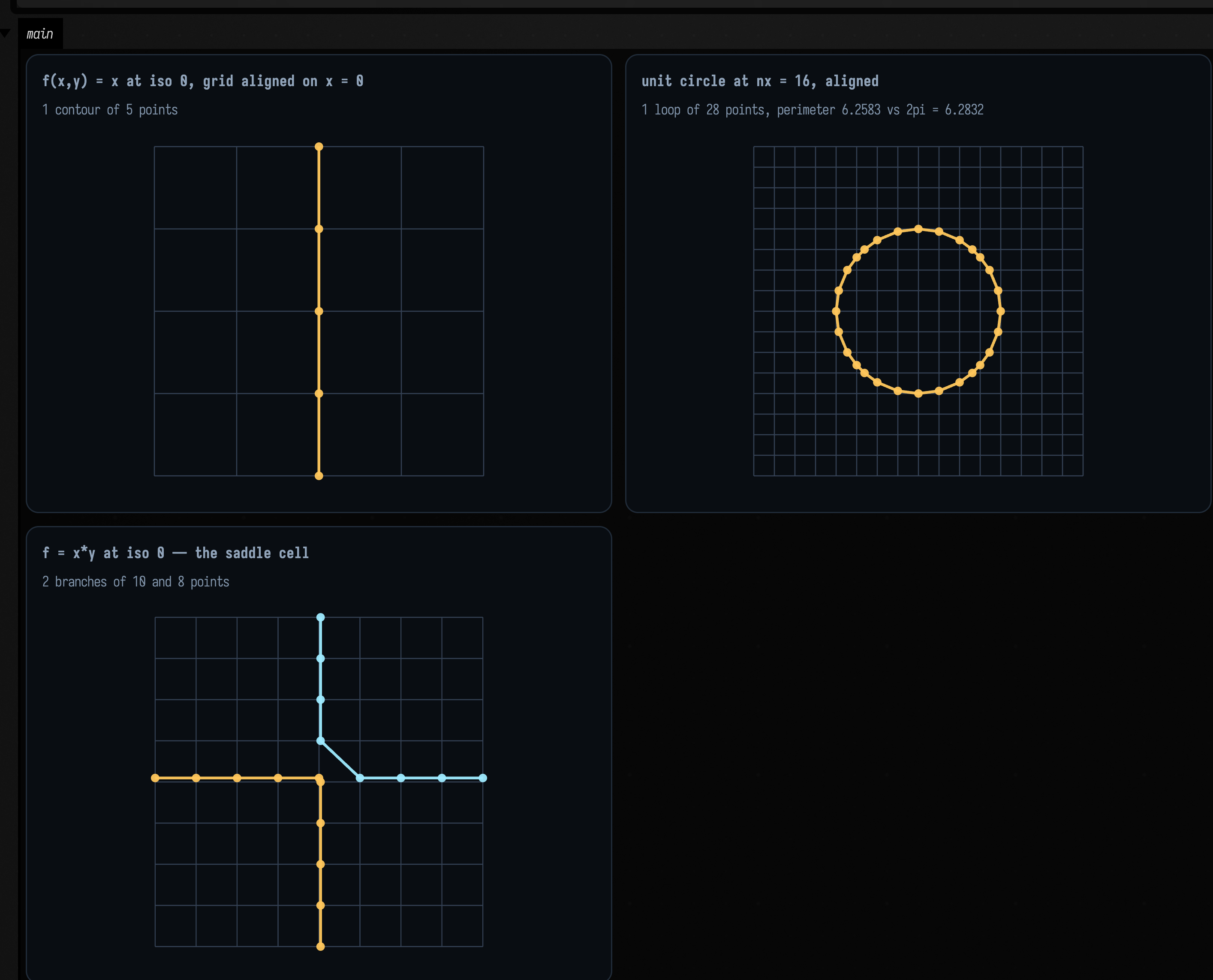
The parenthesised numbers in the captions are what a strict sign-change test returns. f(x, y) = x
at iso = 0 on a grid with an even cell count puts a whole column of samples on the level, and a
strict test gives no contour at all. The unit circle at nx = 16 passes exactly through a grid
corner at each of the four axis points, and a strict test cuts it into four disconnected 6-point
arcs. Field's marcher returns one 5-point line and one closed 28-point loop whose perimeter is
within a percent of 2π.
It uses the same convention as marchingCubes in mesh_sdf.kt, one dimension down:
a corner is inside iff its sample is strictly below iso, so "exactly at iso" is a definite
side rather than a third state, and the crossing parameter is then clamped a thousandth of a cell off
the endpoints so that the several edges out of such a corner do not all interpolate onto the corner
itself. With inside two-valued, a cell can never have an odd number of crossings, so there is no
degenerate case left to handle.
The saddle cell. When the four corners alternate inside/outside there are four crossings and two
ways to pair them, and the two choices give different topology: either the inside region is
connected through the middle of the cell or the outside one is. Picking arbitrarily means two cells
sharing an edge can disagree, and the contour tears there. The resolution is the asymptotic
decider: the cell's bilinear interpolant has exactly one saddle, at value
\( (s_0 s_2 - s_1 s_3) / (s_0 + s_2 - s_1 - s_3) \) with every s measured from iso, and whichever diagonal pair
of corners shares a side with that saddle is the pair the centre connects. It depends only on the
cell's own four corner values, so neighbouring cells always agree, which an arbitrary pairing
cannot guarantee.
The third panel is the case where the decider has nothing to say. \( xy = 0 \) is the two axes
crossing, and a marcher cannot draw an X, so at the saddle cell it joins the four crossings in pairs
and the zero set comes back as two right-angled branches meeting at the origin. But \( xy \) is itself
bilinear, so the cell's interpolant reproduces it exactly and the saddle value is exactly iso. Both
pairings are equally correct, and the decider is looking at a numerator that is zero in exact
arithmetic and ±10⁻²⁰ in doubles, that is, at rounding error. The marcher breaks the tie
deterministically instead, and nx = 8 gives 8 and 10 points. The two branches are not
expected to be equal: the sampling
window is \( [-1.05, 1.03] \times [-1.02, 1.07] \), so the origin sits at cell (4.04, 3.90) and the two arms
of the X are cut by the grid at different places.
The decider matters in any cell whose saddle value is genuinely off iso, and there it reads the
corner magnitudes as well as their signs. Give one cell the values
\( (-3, +1, -3, +1) \): the saddle is at \( -1 \), on the same side as the \( -3 \) diagonal, so those two corners
join through the centre and the crossings cut the two \( +1 \) corners off. Now keep the same sign pattern
and swap which diagonal is the deep one, \( (-1, +3, -1, +3) \). Exactly the same corners are inside, but
the saddle is now \( +1 \), the outside is what joins, and the cuts must move to the other diagonal. An
implementation that looked only at which corners are inside would answer both the same way, drawing
long diagonals across one of the two cells where the decider draws short corner elbows.
There is a matching invariant in the other direction: negating every corner value must leave the crossing exactly where it was. \( \{f = 0\} \) and \( \{-f = 0\} \) are the same set of points, so a marcher that moved the curve would be reporting two different answers for one curve. The two flips cancel: negation swaps which corners are inside and flips the sign of the saddle value, and the decider compares the two.
The next figure shows both the decision and the tie. A single grid cell with four prescribed corner
values is a complete input to generateIsoContours, so the top row feeds it the two cells above;
the bottom row is \( xy \) at two resolutions.
:::static
// A field whose four corner samples are prescribed, on a 1x1 grid: the decider is then the only
// thing under test. v0 bottom-left, v1 bottom-right, v2 top-right, v3 top-left.
fun oneCell(v: List<Double>): ScalarField2D = { x, y ->
    if (x < 0.5) (if (y < 0.5) v[0] else v[3]) else (if (y < 0.5) v[1] else v[2])
}

// The value the decider looks at: the cell's bilinear interpolant has exactly one saddle, and this
// is it. Its SIGN says which diagonal pair of corners the centre of the cell belongs to.
fun saddleValue(v: List<Double>, iso: Double = 0.0): Double {
    val s = v.map { it - iso }
    return (s[0] * s[2] - s[1] * s[3]) / (s[0] + s[2] - s[1] - s[3])
}

// Same sign pattern in both, but the DEEP diagonal moves. That is what the decider reads.
val deepInside = [-3.0, 1.0, -3.0, 1.0] // saddle -1: the inside joins through the centre
val deepOutside = [-1.0, 3.0, -1.0, 3.0] // saddle +1: the outside joins, so the cuts move

val insideCut = generateIsoContours(oneCell(deepInside), 0.0, 1.0, 0.0, 1.0, 1, 1, 0.0)
val outsideCut = generateIsoContours(oneCell(deepOutside), 0.0, 1.0, 0.0, 1.0, 1, 1, 0.0)

/*
The other-direction invariant: {f = 0} and {-f = 0} are the same set of points, so negating every
corner value must NOT move the crossing. It cancels — negation swaps inside/outside AND flips the
saddle's sign, and the decider compares the two.
*/
fun cutCentres(cuts: List<List<Vec2>>) =
    cuts
        .map { c ->
            "%.2f,%.2f".format((c[0].x + c[1].x) / 2.0, (c[0].y + c[1].y) / 2.0)
        }
        .sorted()
val negationIsInvariant =
    [deepInside, deepOutside].all { v ->
        cutCentres(generateIsoContours(oneCell(v), 0.0, 1.0, 0.0, 1.0, 1, 1, 0.0)) ==
            cutCentres(generateIsoContours(oneCell(v.map { -it }), 0.0, 1.0, 0.0, 1.0, 1, 1, 0.0))
    }

/*
f = x*y is the tie, and it is the common case rather than the exotic one: the field is ITSELF
bilinear, so the cell's interpolant reproduces it and the saddle value is exactly iso. Locate the
saddle cell at a given resolution and report the numerator that is supposed to decide it.
*/
fun tieNumerator(nx: Int): Double {
    val dx = (1.03 - -1.05) / nx
    val dy = (1.07 - -1.02) / nx
    for (i in 0 until nx) for (j in 0 until nx) {
        val a = -1.05 + i * dx
        val c = a + dx
        val b = -1.02 + j * dy
        val d = b + dy
        val v = [a * b, c * b, c * d, a * d]
        val alternates = (v[0] < 0) != (v[1] < 0) && (v[1] < 0) != (v[2] < 0) && (v[2] < 0) != (v[3] < 0)
        if (alternates) return v[0] * v[2] - v[1] * v[3]
    }
    return Double.NaN
}

val saddleField: ScalarField2D = { x, y -> x * y }
val tie8 = generateIsoContours(saddleField, -1.05, 1.03, -1.02, 1.07, 8, 8, 0.0)
val tie32 = generateIsoContours(saddleField, -1.05, 1.03, -1.02, 1.07, 32, 32, 0.0)
:::fold draw the cell, its corners by sign, and the crossing it chose
val insideColor = vec(0.42, 0.72, 1.0, 0.95) // strictly below iso — inside
val outsideColor = vec(1.0, 0.62, 0.36, 0.95) // at or above iso — outside
val cutColor = vec(0.6, 1.0, 0.72, 0.95)

fun cellFigure(v: List<Double>, cuts: List<List<Vec2>>): List<FLine> {
    val out = ArrayList<FLine>()
    out += fline {
        rect(0.0, 0.0, 1.0, 1.0)
        color = vec(0.34, 0.42, 0.54, 0.7)
        thickness = 1.0
    }
    val corners = [vec(0.0, 0.0), vec(1.0, 0.0), vec(1.0, 1.0), vec(0.0, 1.0)]
    corners.forEachIndexed { i, p ->
        out +=
            pointCloudFLine(
                [p],
                color = if (v[i] < 0.0) insideColor else outsideColor,
                pointSize = 3.0,
            )
    }
    cuts.forEach { c ->
        out +=
            polylineFrom(c, 0, closed = false).also {
                it.color = cutColor
                it.thickness = 3.2
                it.pointed = true
                it.pointSize = 1.4
            }
    }
    return out
}

fun gridLines(x0: Double, x1: Double, y0: Double, y1: Double, n: Int) = fline {
    grid(Rect(x0, y0, x1 - x0, y1 - y0), n, n)
    color = vec(0.34, 0.42, 0.54, 0.45)
    thickness = 0.7
}

fun branchLines(contours: List<List<Vec2>>): List<FLine> {
    val palette = [vec(1.0, 0.78, 0.36, 0.95), vec(0.62, 0.92, 1.0, 0.95)]
    return contours.mapIndexed { i, c ->
        polylineFrom(c, 0, closed = false).also {
            it.color = palette[i % palette.size]
            it.thickness = 2.4
            it.pointed = true
            it.pointSize = 1.1
        }
    }
}

fun sizes(contours: List<List<Vec2>>) = contours.map { it.size }.joinToString(" and ")

// Captions stay short: showPlaneGrid lays the cards out on `max-content`, so a long
// single-line caption widens the card past the docs screenshot's ~1100 CSS px crop and gets cut off.
showPlaneGrid(
    "−3 / +1 / −3 / +1   deep inside\nsaddle ${"%+.3f".format(saddleValue(deepInside))} — cuts isolate the shallow pair" to
        cellFigure(deepInside, insideCut),
    "−1 / +3 / −1 / +3   deep outside\nsaddle ${"%+.3f".format(saddleValue(deepOutside))} — same signs, other diagonal" to
        cellFigure(deepOutside, outsideCut),
    "f = x·y at nx = 8 — a genuine tie\nnumerator ${"%+.1e".format(tieNumerator(8))} = zero; ${sizes(tie8)} points" to
        ([gridLines(-1.05, 1.03, -1.02, 1.07, 8)] + branchLines(tie8)),
    "…at nx = 32, same tie, same pairing\nnumerator ${"%+.1e".format(tieNumerator(32))}; ${sizes(tie32)} points" to
        ([gridLines(-1.05, 1.03, -1.02, 1.07, 32)] + branchLines(tie32)),
    columns = 2,
    cellWidth = 430,
    cellHeight = 260,
)
println("negating every corner value leaves the crossing put: $negationIsInvariant")
:::endfold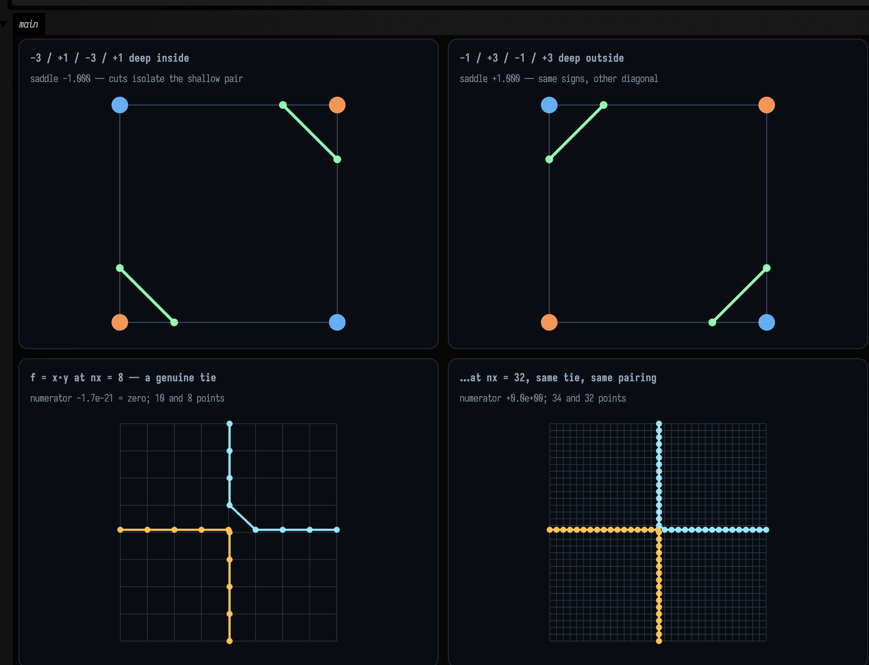
In the top row the two cells have the same sign pattern, with the same two corners inside, and
the crossings still land on opposite diagonals. All that changed is which diagonal is the deep
one, and therefore which side of iso the saddle falls on. Only the four corner values decide the
pairing, which is what lets two cells sharing an edge agree about the crossing on it.
The box also prints the negation check: negating every corner value leaves the crossing exactly
where it was, as it must, because {f = 0} and {−f = 0} are the same curve.
In the bottom row the decider has nothing to go on. The numerators in the captions, -1.7e-21 and
0.0, are both zero, so the saddle is exactly on iso, the level set through that cell is an X
meeting at a point, and both pairings are equally correct. Left to the numerator's sign, the pairing
would depend on which way a multiplication rounded, and could change with grid resolution. The two
panels agree because the marcher settles the tie with SADDLE_TIE_RELATIVE_EPSILON instead.
Sweep the level through the saddle
The saddle cell matters because of what happens to the whole level set when the iso level passes through a saddle: its topology changes at that one level, which a still image cannot show.
This example uses two Gaussian bumps and sweeps the iso level from 0.18 up to 0.78 and back. The
col (the low point of the ridge between the two peaks) sits at 0.391, computed in the box as
field(0.0, 0.0), and is marked in orange. Below it there is one contour enclosing both peaks;
above it there are two, one per peak. Each contour is coloured by its index, so you see the
merge as a colour vanishing as well as in the caption's count.
:::static
:::fold two Gaussian bumps, the sampling window, the palette, and the clock
val field: ScalarField2D = { x, y ->
    exp(-((x - 1.4) * (x - 1.4) + y * y) / 1.2) + exp(-((x + 1.4) * (x + 1.4) + y * y) / 1.2)
}
// The sampled rectangle, and a FIXED display window so the picture does not rescale as the loops
// shrink — the contours would otherwise stay the same size on screen and the sweep would look still.
val x0 = -3.2
val x1 = 3.2
val y0 = -1.9
val y1 = 1.9
val window = Rect(-3.0, -1.7, 6.0, 3.4)
val peakDots = pointCloudFLine(
    [vec(1.4, 0.0), vec(-1.4, 0.0)],
    color = vec(1.0, 1.0, 1.0, 0.85),
    pointSize = 1.4,
)
val saddleDot = pointCloudFLine(
    [vec(0.0, 0.0)],
    color = vec(1.0, 0.72, 0.32, 0.98),
    pointSize = 1.9,
)
val byIndex = [vec(0.42, 0.80, 1.0, 0.95), vec(1.0, 0.45, 0.62, 0.95)]
// Match the eight-second fence: offline capture advances this clock by exactly 1 / fps per frame.
val sweepSeconds = 8.0
val started = AnimationClock.nowSeconds()
:::endfold

// The saddle level is the field's own value at the col between the peaks.
val saddle = field(0.0, 0.0)

/*
The line that turns elapsed time into the swept parameter. A triangle ramp over a range that
straddles `saddle` with room either side, so the topology change happens twice per loop, once each
way.
*/
fun isoAt(elapsed: Double): Double {
    val phase = (elapsed / sweepSeconds) % 1.0
    return 0.18 + 0.60 * (1.0 - abs(1.0 - 2.0 * phase)) // 0.18 -> 0.78 -> 0.18
}

animate {
    val iso = isoAt(AnimationClock.nowSeconds() - started)
    // This resolution controls geometry cost and detail; capture speed cannot stretch the sweep.
    val contours = generateIsoContours(field, x0, x1, y0, y1, 100, 60, iso).filter { it.size >= 2 }
    val lines = contours.mapIndexed { i, c ->
        polylineFrom(c, 0, closed = isoContourClosed(c, x0, x1, y0, y1, boundaryEpsilon = 0.05)).also {
            it.color = byIndex[i % byIndex.size]
            it.thickness = 2.0
        }
    }
    showPlane(
        lines + peakDots + saddleDot,
        title = "iso %.3f — %d contour(s)".format(iso, contours.size),
        caption =
            if (iso > saddle) "above the saddle %.3f — one loop per peak".format(saddle)
            else "below the saddle %.3f — one loop around both".format(saddle),
        width = 660,
        height = 374,
        window = window,
    )
}
Partitioning the cloud instead of the plane
The last family asks the question the other way round: not "which part of the plane belongs to which point" but "which points belong together".
There is no k-means in Field, by design. Every algorithm in clustering.kt returns either a
hierarchy or a centre that is meaningful for the data it summarises. A medoid is one of your
own samples: the actual document, the actual frame, the actual brush mark. A median is
coordinate-wise robust. A k-means centroid is neither, and on a cloud with one outlier it is the one
that moves. The three entry points:
val tree = vec2Agglomerative(points, AgglomerativeLinkage.WARD) // the whole merge hierarchy
tree.partition(k) // cut it at k clusters -> ClusterLayer
tree.partitionByHeight(h) // …or at a merge distance
tree.layers(2..6) // …or at several k at once

vec2KMedoids(points, k, KMedoidsOptions(randomSeed = 11L)) // centres ARE samples
vec2KMedians(points, k, KMediansOptions(randomSeed = 11L)) // L1 Lloyd, robust centres
Each of Float, Vec2, Vec3 and Vec4 has all three (floatKMedoids, vec3Agglomerative, …),
and every result converts to a ClusterLayer, a name plus one integer label per sample, which is
the form the visualisers take.
On three well-separated Gaussian blobs every strategy below gives the same answer, so the example adds one complication: three tight blobs of 28 points, plus a single 85th point nine units away from all of them. Watch what each strategy does with that one point.
:::fold plant three tight blobs of 28 — and one lone stray nine units out
// Three tight Gaussian blobs, 28 points each, centres 2.4 apart. Then one stray, far from all three.
// The only interesting thing about this cloud is that 85th point.
val rng = java.util.Random(7)
val blobCentres = [vec(0.0, 0.0), vec(2.4, 0.2), vec(1.2, 2.2)]
val blobs = blobCentres.flatMap { c ->
    List(28) { vec(c.x + rng.nextGaussian() * 0.30, c.y + rng.nextGaussian() * 0.30) }
}
val stray = vec(9.0, 8.0)
// NOT `blobs + stray`: in Field, `List<Vec2> + Vec2` is `FLineGeometry`'s elementwise operator and
// TRANSLATES all 84 points by (9, 8) rather than appending an 85th. `+ [stray]` is worse still
// — that overload zips two equal-length lists. Append explicitly.
val points = buildList { addAll(blobs); add(stray) }
val window = Rect(-1.4, -1.4, 11.2, 10.2)   // shared by all four panels, so they are comparable
:::endfold
:::static
// Four strategies, one question: partition these 85 points into three groups.
val tree = vec2Agglomerative(points) // Ward: minimises within-cluster sum of SQUARES
val cut3 = tree.partition(3)
val cut6 = tree.partition(6)
val medoids = vec2KMedoids(points, 3, KMedoidsOptions(randomSeed = 11L)) // centres ARE samples
val medians = vec2KMedians(points, 3, KMediansOptions(randomSeed = 11L)) // L1 Lloyd

// One ruler for all of them: score ANY partition by the objective k-medians optimises — the sum of
// |dx| + |dy| from each point to its own cluster's median. That makes the four answers comparable.
fun l1Of(labels: IntArray, k: Int) =
    (0 until k).sumOf { c ->
        val mem = points.indices.filter { labels[it] == c }
        val mx = mem.map { points[it].x }.sorted()[mem.size / 2]
        val my = mem.map { points[it].y }.sorted()[mem.size / 2]
        mem.sumOf { (abs(points[it].x - mx) + abs(points[it].y - my)).toDouble() }
    }
fun sizes(layer: ClusterLayer) = (0 until layer.clusterCount).map { layer.indices(it).size }.sorted()

// THE DISCRIMINATORS. Every one of these is boring on well-separated blobs and decisive here.
val wardSpendsAClusterOnTheStray = sizes(cut3).first() == 1 // [1, 28, 56]
val medoidsKeepEveryBlobWhole = medoids.clusterSizes.min() >= 28 // [28, 28, 29]
val wardCostsThisMuchMore = l1Of(cut3.labels, 3) / medians.objective // 1.86x, not 1.00x

// …and the invariants that hold whatever the data, which is why they are the backbone.
val medoidsAreSamples = medoids.medoids.all { m -> points.any { it.x == m.x && it.y == m.y } }
val nested =
    (0 until cut6.clusterCount).all { fine ->
        cut6.indices(fine).map { cut3.labels[it] }.toSet().size == 1
    }
val mediansBeatMedoids = medians.objective < medoids.distortion
:::fold draw the four partitions
// Only the FIRST newline splits a panel label into title + caption; later ones render as spaces, and
// the grid's max-content columns are sized by the longest caption. So: one short caption line each.
showPlaneGrid(
    "vec2Agglomerative().partition(3)\nsizes ${sizes(cut3).joinToString("/")} — L1 %.3f. one stray, one whole cluster"
        .format(l1Of(cut3.labels, 3)) to cut3.toFLines(points, drawSpokes = false, pointSize = 1.6),
    "…the SAME tree, cut at 6\nsizes ${sizes(cut6).joinToString("/")} — nested: $nested. the blobs are back" to
        cut6.toFLines(points, drawSpokes = false, pointSize = 1.6),
    "vec2KMedoids(k = 3)\nsizes ${medoids.clusterSizes.toList().sorted().joinToString("/")} — distortion %.3f. samples: %s"
        .format(medoids.distortion, medoidsAreSamples) to
        medoids.asLayer().toFLines(points, centers = medoids.medoids, pointSize = 1.6),
    "vec2KMedians(k = 3)\nsizes ${medians.clusterSizes.toList().sorted().joinToString("/")} — L1 %.3f. Ward's cut costs %.2fx"
        .format(medians.objective, wardCostsThisMuchMore) to
        medians.asLayer().toFLines(points, centers = medians.centers, pointSize = 1.6),
    columns = 2,
    cellWidth = 430,
    cellHeight = 352,
    window = window,
)
:::endfold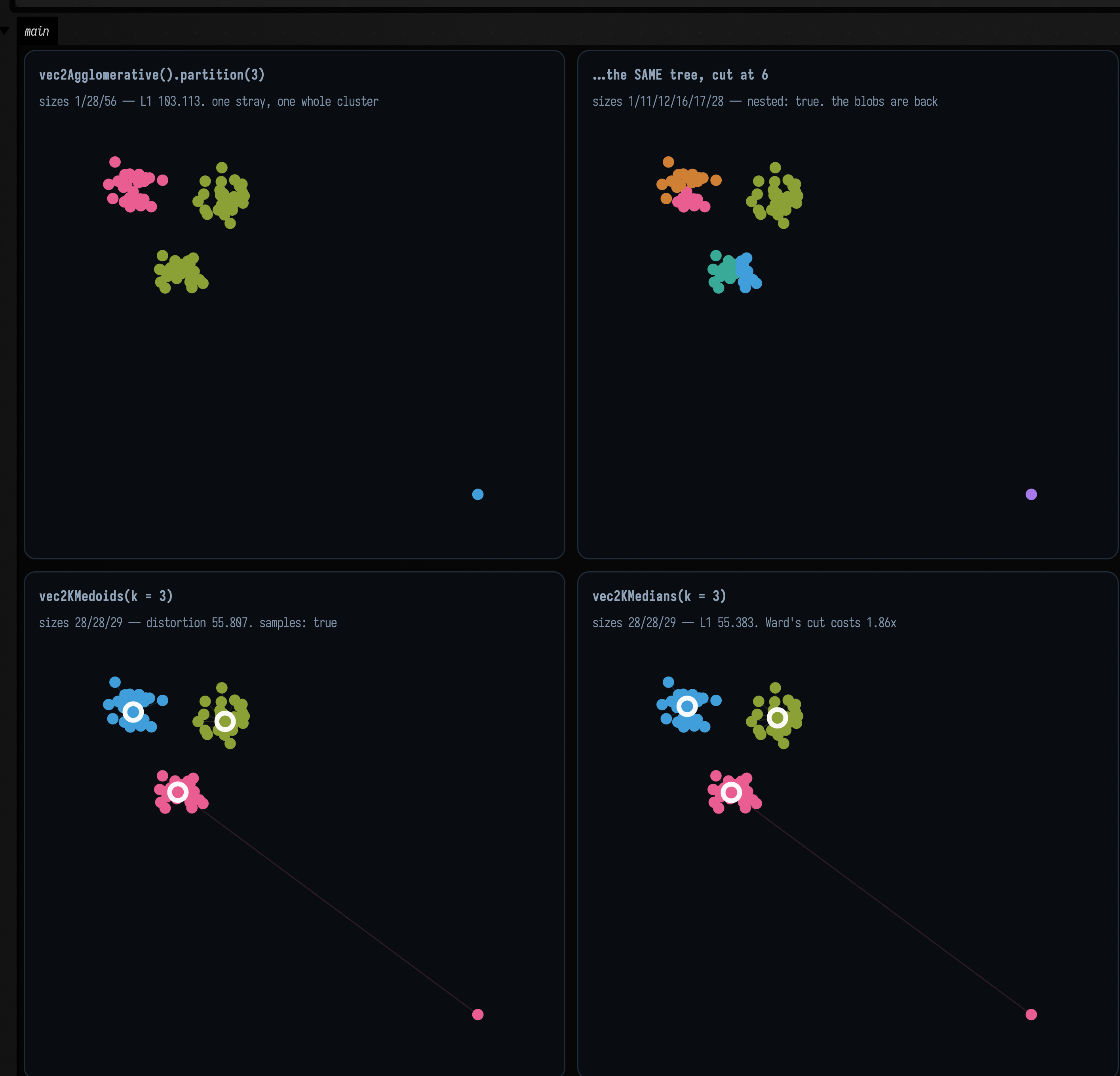
The four strategies disagree, and each disagreement is a reason to pick one over another.
Ward spends a whole cluster on one point. The k=3 cut is 1 / 28 / 56: the stray alone, one blob
intact, and two genuine blobs merged into one. That follows from Ward's objective. Agglomerative
Ward merges whichever pair raises the within-cluster sum of squares least, and merging clusters of
\( n_1 \), \( n_2 \) whose centroids are d apart costs \( \frac{n_1 n_2}{n_1 + n_2} d^2 \). Merging two 28-point blobs 2.408
apart costs \( 14 \cdot 5.80 = 81.2 \). Absorbing the stray into its nearest blob (9.72 away) costs
\( \tfrac{28}{29} \cdot 94.5 = 91.2 \). 91.2 > 81.2, so the stray stays out and two real clusters pay for it. It
all comes from the squaring: a point three times further away is nine times as expensive.
The same arithmetic predicts where the behaviour changes: at \( d = \sqrt{81.2 / 0.966} = 9.17 \). Moving the
stray inward, the cut flips from 1 / 28 / 56 to 28 / 28 / 29 between d = 8.32 and d = 9.72,
the two sampled distances that bracket 9.17.
k-medoids and k-medians both absorb the stray, and here they give the right answer. Both minimise a sum of distances, so that point costs 9.72 rather than 94.5, and absorbing it as one eccentric member of the nearest blob is much cheaper than splitting a real blob apart. Both return 28 / 28 / 29, both recover all three planted blobs whole, and every medoid is still one of your own samples. Scored on one ruler, the L1 objective in the code above, Ward's cut costs 103.113 where k-medians reaches 55.383: 1.86× as much.
The hierarchy is the only one of the four you can revisit after the fact. Cut the same tree at 6 and you get 1 / 11 / 12 / 16 / 17 / 28: the stray is a singleton, and the two blobs Ward merged at k=3 are separate again. Every planted blob is a union of k=6 clusters even though the k=3 cut ran across them. That costs nothing (no re-run, no re-seed, no new random number) because the finer cut is nested inside the coarser one. So k-medoids and k-medians give a better answer to the question you asked, and the hierarchy lets you discover you asked the wrong question.
Two more things about vec2KMedoids:
- It is Field's own implementation, the alternating algorithm, beside the k-medians in
clustering.kt, with D²-weighted seeding andrunsrestarts, so arandomSeedmakes it reproducible. - It is O(n²) in memory, because it precomputes the full distance matrix. Fine for thousands of points; not for millions.
Why not Smile's KMedoids
Smile 5's KMedoids is CLARANS and floors an internal maxNeighbor at min(100, k·(n−k)),
reachable through no option, then rejects any value above n, so for \( k \ge 2 \) it throws
IllegalArgumentException: Too large maxNeighbor: 100 for every sample count below about a
hundred.
The linkage is the model
One stray point was enough to separate the three algorithms. It is not enough to separate the seven
AgglomerativeLinkage values, because all seven agree that a lone far point is its own cluster. They
disagree about what a cluster is, and showing that needs a shape rather than an outlier.
The example uses two long parallel bands with a narrow gap and a few stragglers in it, a standard test because it separates the two rival definitions of "cluster". One is connectivity: a set of things each close to something in the set, which follows an elongated shape wherever it goes. The other is compactness: a set of things all close to each other, which prefers a blob and will break an elongated shape rather than accept it. Single linkage is the first; complete, Ward and the averages are the second.
:::static
// Two long bands with a narrow gap, plus three stragglers sitting in the gap — a chain waiting to
// happen. n = 83, and there is no "right" answer, which is the point.
val rng = java.util.Random(23)
val band = { y0: Double ->
    (0 until 40).map { i -> vec(i * 0.25 + rng.nextDouble() * 0.1, y0 + rng.nextDouble() * 0.28) }
}
val bridge = [vec(4.4, 0.62), vec(4.9, 0.78), vec(5.4, 0.95)]
// NB `flatten()`, not `+`: on List<Vec2> the plus operator is *elementwise vector addition*, so
// `band(0.0) + bridge` is an IllegalArgumentException about mismatched list sizes, not a concat.
val banded = [band(0.0), band(1.5), bridge].flatten()

// Every linkage, cut at the same k. The ONLY thing that varies between panels is the linkage.
val cuts =
    AgglomerativeLinkage.entries.map { linkage ->
        linkage to vec2Agglomerative(banded, linkage).partition(3)
    }

// The discriminator, as a number rather than an impression: how big is the largest cluster? A
// chaining linkage swallows nearly everything into one, and leaves singletons behind.
val largest = cuts.associate { (l, cut) ->
    l to (0 until cut.clusterCount).maxOf { cut.indices(it).size }
}
val singletons = cuts.associate { (l, cut) ->
    l to (0 until cut.clusterCount).count { cut.indices(it).size == 1 }
}

/*
Single linkage's notorious failure mode is chaining across a gap. Does it happen HERE? Drop to
k = 2 and read the largest cluster: 82-ish would mean the chain crossed the gap through the
stragglers, 43 means it did not and the two bands survived.
*/
val singleAtTwo = vec2Agglomerative(banded, AgglomerativeLinkage.SINGLE).partition(2)
val singleAtTwoLargest = (0 until singleAtTwo.clusterCount).maxOf { singleAtTwo.indices(it).size }
:::fold draw the input and all seven cuts
fun panel(cut: ClusterLayer) = cut.toFLines(banded, drawSpokes = false, pointSize = 1.5)

val inputPanel = [pointCloudFLine(banded, color = vec(1.0, 1.0, 1.0, 0.85), pointSize = 1.5)]
val frame = Rect(-0.4, -0.4, 10.6, 2.6)

showPlaneGrid(
    "the input — 83 points, k = 3\ntwo bands of 40 plus 3 stragglers in the gap" to inputPanel,
    *cuts
        .map { (linkage, cut) ->
            // The k=2 note rides on SINGLE's own caption, so the number the prose quotes is visible in
            // the figure rather than only in a printed line the screenshot crop may not reach.
            val extra = if (linkage == AgglomerativeLinkage.SINGLE) "; at k=2, $singleAtTwoLargest" else ""
            "$linkage\nlargest cluster ${largest[linkage]} of 83, ${singletons[linkage]} singleton(s)$extra" to
                panel(cut)
        }
        .toTypedArray(),
    columns = 2,
    cellWidth = 430,
    cellHeight = 132,
    window = frame,
)
println(
    "SINGLE at k=2: largest cluster $singleAtTwoLargest of ${banded.size} — the chain crossed the gap",
)
:::endfold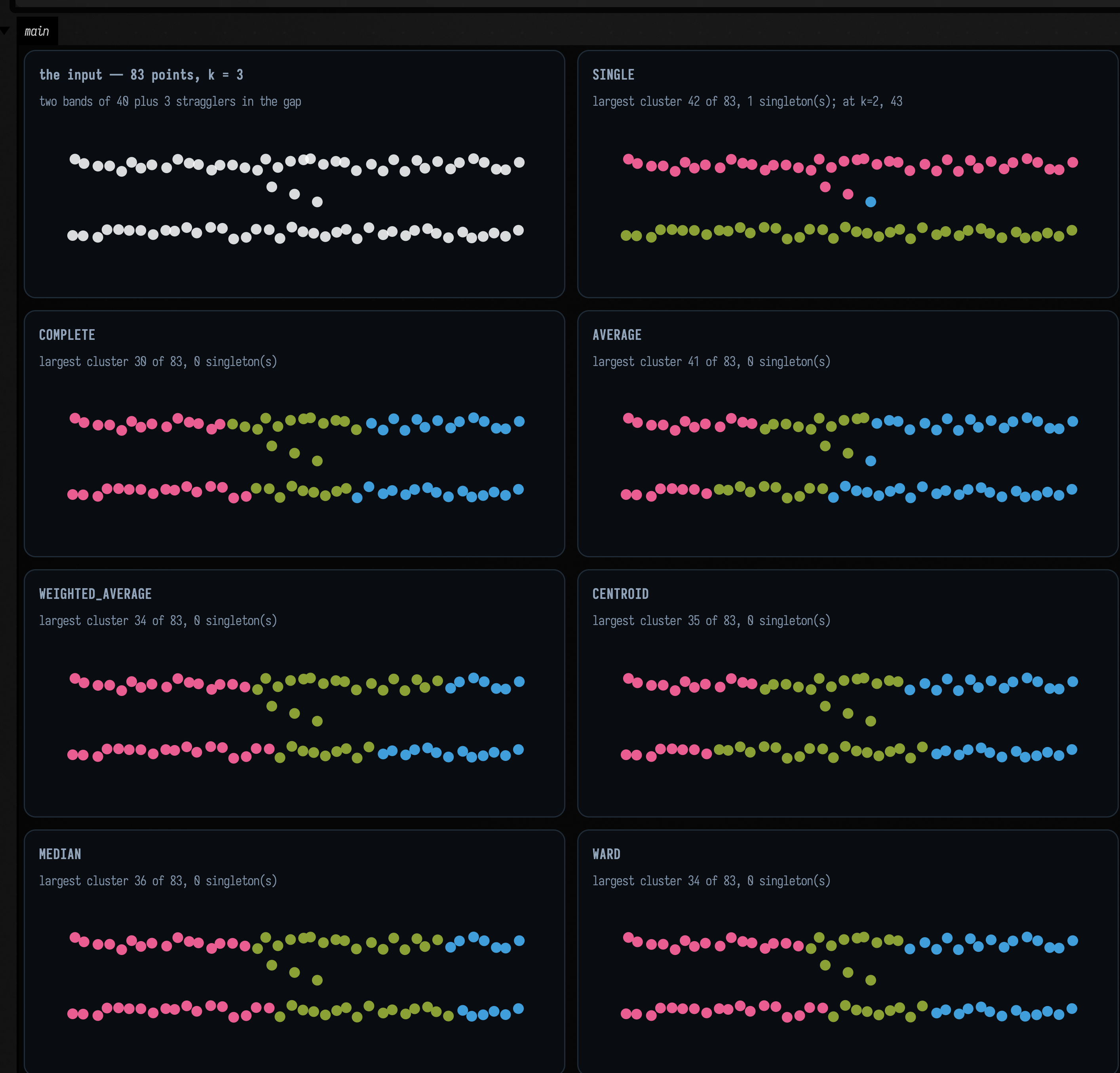
SINGLE is the only one of the seven that finds the bands, which is the opposite of single
linkage's reputation. It returns one band of 40, the other band plus two of the stragglers as 42,
and the remaining straggler as a singleton. Every other linkage ignores the gap entirely and cuts
both bands into three vertical slabs (pink, green, blue left to right) because for a compactness
criterion a 10-by-0.3 band is not a cluster at all, and three slabs are rounder than two bands.
Neither is the better setting. They answer different questions, and the gap in this data is narrower than the bands are long, so "close" genuinely means two different things here.
Single linkage is known for chaining: a thin bridge of points lets it merge two groups that are
nowhere near each other. This data has a bridge, three stragglers sitting in the gap, and still the
two bands stay apart at k = 2. The number after the semicolon in SINGLE's caption is the largest
cluster at k = 2, and it is 43, not 82: the third straggler joins the band it was already
nearest.
Here the bridge is too sparse to join the bands early. Along a band the
nearest-neighbour spacing is about 0.25; the shortest hop from a straggler to the far band is about
0.55. Single linkage merges the cheapest pair available at every step, so every within-band link is
used up long before any gap-crossing one, and there is no k at which the chain wins. It takes
single linkage and a finely sampled bridge.
The practical reading: reach for WARD (the default) when you want compact groups of similar size,
SINGLE when you are looking for connected filaments and want to follow them, COMPLETE when one
outlier must not be allowed to merge two real groups, and AVERAGE when you have no opinion.
CENTROID and MEDIAN can produce inversions (a merge at a lower height than one of its children),
so a dendrogram drawn from them is not monotone. Every implementation of those two methods does
this.
There is also a visualizeVec2ClusterLayers3D(points, layers) (and Vec3/Float siblings, and
tree.visualizeVec2(2..6)) which stacks several ClusterLayers along one axis into a 3D drawing
of the hierarchy: the whole ladder of k at once, for threeLines(...) rather than a flat figure.
It returns FLines keyed "cluster-points", "cluster-points-halo", "cluster-centers",
"cluster-centers-halo", "cluster-links", "cluster-guides".
Up one dimension
voronoi.kt does the exact unweighted construction in 3D, by half-space clipping: for each site,
intersect the bisector half-space against every other site's, plus six clip planes, and keep the
polyhedron. voronoi3d(points) returns a VoronoiLattice of VoronoiCell3s, each a list of
VoronoiFaces with a polygon and the neighbour it faces.
val lattice = voronoi3d(sites) // or Voronoi3d.build(sites, tolerance, clipPadding)
lattice[7].faces // List<VoronoiFace>
face.neighborSite // null for a clip-box face
face.polygon // wound CCW along face.plane.normal
cell.bounded // false if any face is a clip face or touches the box
A 3D diagram is a different object from the 2D one. The two live in different files and the
names do not warn you: a plane slice through a 3D Voronoi diagram is not
the 2D Voronoi diagram of the sites projected onto that plane. The slice's cells are bounded by the
bisectors of 3D distances, so a site far above or below the slice plane still owns territory in it, and two sites that look adjacent from above may not
share a face at all. If what you want is the flat thing, you want
graph_connectivity.kt and vec2VoronoiDiagram, JTS-backed and
exact, not this file.
The figure slices a random 48-site 3D diagram, draws the 2D diagram of the same sites flattened beside it, and slices a cubic lattice whose answer is known in advance.
:::static
/*
48 sites in a 3-cube, and the 3D diagram of them. The 3-cube is chosen so that the cubic lattice
below — 4x4x4 sites one unit apart — occupies exactly the same window, and all three panels of the
figure can therefore share one scale.
*/
val rng = java.util.Random(11)
val sites3 = List(48) { vec(rng.nextDouble() * 3.0, rng.nextDouble() * 3.0, rng.nextDouble() * 3.0) }
val lattice = voronoi3d(sites3)

// Every cell must contain its own site — the defining property, and cheap to check: the site is on
// the inside of every one of the cell's face planes.
val siteInsideOwnCell =
    lattice.cells.all { cell ->
        cell.faces.all { f ->
            val n = f.plane.normal
            n.x * cell.site.x + n.y * cell.site.y + n.z * cell.site.z <= f.plane.d + 1e-3f
        }
    }

/*
A cubic lattice is the case with an answer known in advance: 4x4x4 sites one unit apart, so the
eight interior cells must be exact unit cubes — six faces each — and any plane through one of them
must cut it in a 1x1 square. z = 1.2 is chosen to pass through the middle of the lower layer of
them rather than along the boundary between layers, which z = 1.5 would.
*/
val cubic =
    (0 until 4).flatMap { i ->
        (0 until 4).flatMap { j ->
            (0 until 4).map { k ->
                vec(i.toDouble(), j.toDouble(), k.toDouble())
            }
        }
    }
val cubicLattice = voronoi3d(cubic)
val interiorCubes = cubicLattice.cells.count { c -> c.bounded && c.faces.size == 6 }

// …and the 2D diagram of the same sites, flattened. Different object, and the picture says so.
val flattened = sites3.map { vec(it.x.toDouble(), it.y.toDouble()) }
val flat2d = vec2VoronoiDiagram(flattened)
:::fold slice each 3D cell at the selected z levels, and draw
// A convex polygon meets a plane in at most one segment: walk its edges, keep the two crossings.
fun sliceOf(cell: VoronoiCell3, z0: Double): FLine? {
    val segments = ArrayList<Pair<Vec2, Vec2>>()
    for (face in cell.faces) {
        val poly = face.polygon
        if (poly.size < 3) continue
        val hits = ArrayList<Vec2>()
        for (i in poly.indices) {
            val a = poly[i]
            val b = poly[(i + 1) % poly.size]
            val za = a.z.toDouble()
            val zb = b.z.toDouble()
            if ((za < z0) == (zb < z0)) continue
            val t = (z0 - za) / (zb - za)
            hits += vec(a.x + t * (b.x - a.x), a.y + t * (b.y - a.y))
        }
        if (hits.size == 2) segments += hits[0] to hits[1]
    }
    if (segments.isEmpty()) return null
    return fline {
        segments.forEach { (a, b) ->
            moveTo(a.x.toDouble(), a.y.toDouble())
            lineTo(b.x.toDouble(), b.y.toDouble())
        }
        thickness = 1.6
    }
}

/*
Bounded cells only. An unbounded cell's clip-box faces are as large as the clip box (which is
`clipPadding * scale + 1` on every side, so much larger than the sites), and slicing them draws
rays across the whole panel that say nothing about the tiling.
*/
fun sliceLines(l: VoronoiLattice, z0: Double, palette: List<Vec4>): List<FLine> =
    l.cells
        .filter { it.bounded }
        .mapIndexedNotNull { i, cell ->
            sliceOf(cell, z0)?.also { it.color = palette[i % palette.size] }
        }

// "The slice is a square grid", as a check: every slice of an interior cube must have a
// 1x1 bounding box.
fun sliceIsUnitSquare(cell: VoronoiCell3, z0: Double): Boolean {
    val line = sliceOf(cell, z0) ?: return false
    val b = line.fast2DBounds()
    return abs(b.w - 1.0) < 1e-3 && abs(b.h - 1.0) < 1e-3
}
val cubicSliceCells = cubicLattice.cells.filter { it.bounded && sliceOf(it, 1.2) != null }
val allUnitSquares = cubicSliceCells.isNotEmpty() && cubicSliceCells.all { sliceIsUnitSquare(it, 1.2) }

val warm = okhslSet(9, saturation = 0.72, lightness = 0.66)
val cool = okhslSet(9, saturation = 0.5, lightness = 0.72)

val sliced = sliceLines(lattice, 1.5, warm)
val cubicSlice = sliceLines(cubicLattice, 1.2, cool)

val flatLines =
    [
            flat2d.toFLines(),
            [pointCloudFLine(flattened, color = vec(1.0, 0.9, 0.5, 0.9), pointSize = 1.6)],
        ]
        .flatten()
// One window for all three panels, so they are directly comparable and no stray clip-box line can
// set the scale.
val sliceWindow = Rect(-0.25, -0.25, 3.5, 3.5)

showPlaneGrid(
    "voronoi3d(48 sites), sliced at z = 1.5\n${sliced.size} bounded cells meet the plane, of ${lattice.cells.size}" to
        sliced,
    "vec2VoronoiDiagram, same sites flattened\n${flat2d.cells.size} cells — a different partition" to flatLines,
    "4x4x4 unit cubic lattice, sliced at z = 1.2\n${cubicSlice.size} slices, each a 1x1 square: $allUnitSquares" to
        cubicSlice,
    columns = 2,
    cellWidth = 430,
    cellHeight = 300,
    window = sliceWindow,
)
println("every cell contains its own site: $siteInsideOwnCell")
println(
    "interior cells that are bounded six-face cubes: $interiorCubes of ${cubicLattice.cells.size}",
)
:::endfold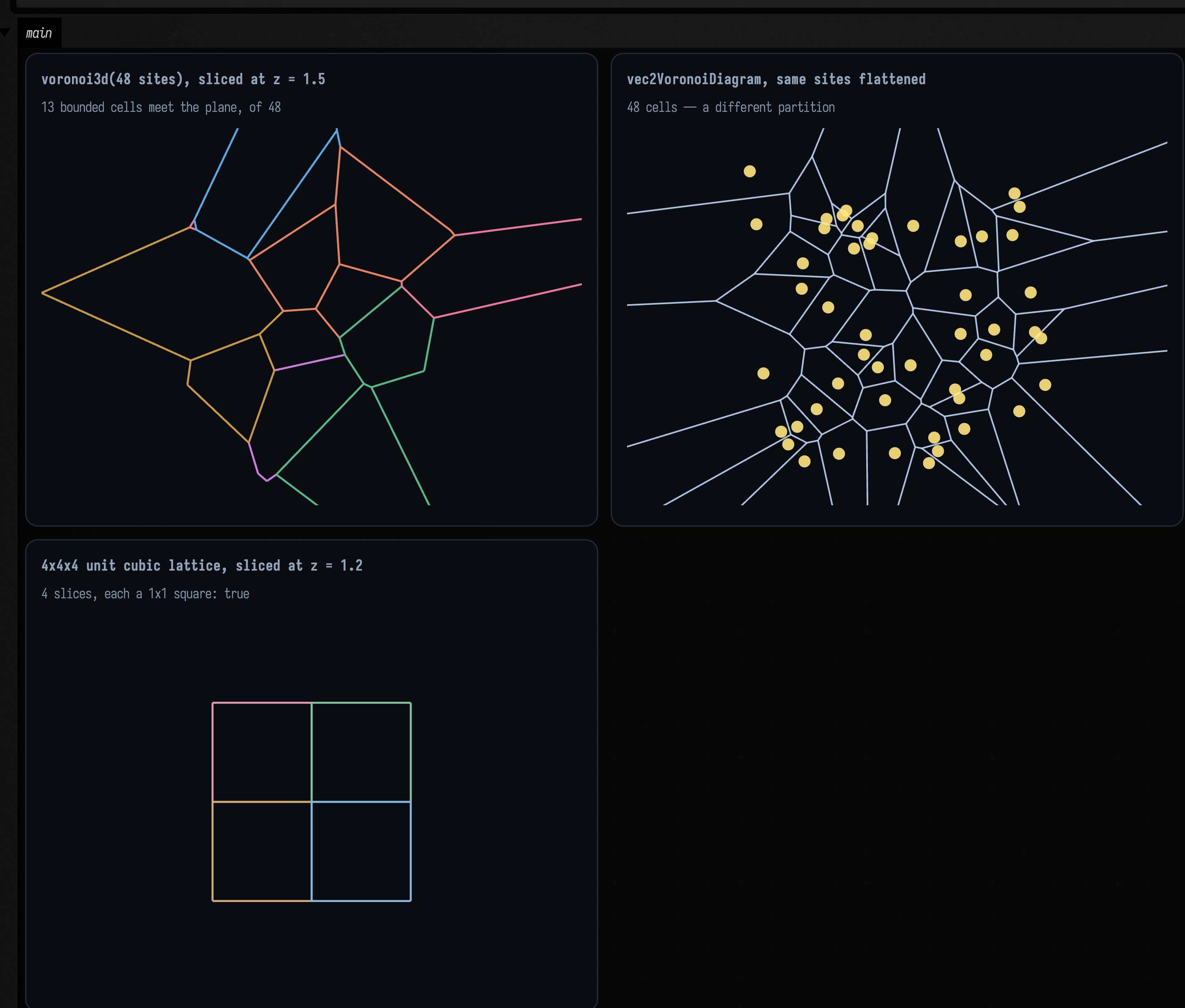
The top two panels show the same 48 points in the same square, partitioned two different ways. Both are correct; they answer different questions. Only the bounded cells are drawn in the slice, because an unbounded cell's clip-box faces are as big as the clip box and slicing them draws rays across the whole panel that say nothing about the tiling.
The third panel has an answer known in advance: 4 × 4 × 4 sites one unit apart, whose eight interior
cells must be exact unit cubes, so a plane through them must cut 1 × 1 squares. The caption reports
that as a measured boolean, every slice's bounding box within 10⁻³ of 1 × 1. Only the cells the
plane actually passes through are drawn, and z = 1.2 rather than 1.5, because 1.5 is exactly
the boundary between two layers of cells and would slice them degenerately.
How face membership is decided is the same problem as the 2D marcher's exact-iso corner. The obvious rule (a corner is on a face if it is within some tolerance of that face's plane) is wrong where four or more bisectors nearly meet, which happens whenever five sites are near-cospherical, and that is common: about a third of the interior cells of a 72-site random lattice have such a corner. The genuine corners near such a cluster are separated by less than any tolerance scaled off the point cloud, so every face passing near the cluster claims every corner in it. The result is a T-junction: a 4.5 × 10⁻³-long edge listed by four faces, and the two long edges radiating from its ends listed by one each. That is a hairline crack in any mesh built from those faces, and no weld tolerance repairs it, because the defect is a face claiming a corner that is not on it.
Membership is instead combinatorial: a corner records which three planes produced it, and a face's polygon is exactly the corners recording that plane. A second pass adds a plane that passes through a corner within that corner's own uncertainty (from a first-order error bound on Cramer's rule), which is what handles exactly symmetric input, where seven bisectors really do meet at each corner of a cubic lattice cell.
Limits. This is a Float clipper and the guarantee is not absolute. Over a sweep,
4 of 465 bounded cells and 12 of 447 clipped cells fail the strict closure check
(every edge walked by exactly two faces in opposite directions). Cell volumes tile the clip box to 1 × 10⁻⁴ relative, and cells
of a cubic lattice come out as exact unit cubes. If you are building a mesh from the faces, use
VoronoiCell3.toTriMesh(shrink) / VoronoiLattice.toTriMesh(...) from
Meshes & 3D Geometry, which is where the pictures of 3D cells live and where the
bridge does its own repair.
Recipes
| Task | Call | What to expect |
|---|---|---|
| the Voronoi cells of some points | vec2VoronoiDiagram(points).toFLines() |
Partitions the plane by nearest site and converts the cell boundaries to line geometry. |
| the Delaunay triangulation | vec2DelaunayGraph(points).toFLine(points) |
Builds Delaunay adjacency and draws its edges. Use the triangle helper when the faces themselves matter. |
| its faces, not its edges | delaunayTrianglesToFLine(points, vec2DelaunayTriangles(points)) |
Converts triangulation faces into line geometry. The input points remain the coordinate source for the indexed triangles. |
| the outline of a point set | polylineFrom(vec2ConvexHull(points).hullPoints, closed = true) |
Finds the convex envelope and closes it as a polyline. Concavities in the original point set are not retained. |
| Voronoi with sites of different importance | CircularDirichlet.build(sites).toFLines(clip = box) |
Builds multiplicatively weighted cells with curved boundaries. A clip box makes unbounded cells drawable. |
| …one cell of it, as arcs you can inspect | diagram[i].pieces.map { it.support } |
Exposes the supporting circle or line for each boundary piece. This preserves analytic geometry before tessellation. |
| soft, rounded Voronoi cells | contour \( d_2 - d_1 \) at a positive iso level (zero finds nothing) | Contours the gap between the two nearest-site distances. A positive level gives rounded inset cells; zero has no interior band to extract. |
| the level set of any 2D function | generateIsoContours(field, xMin, xMax, yMin, yMax, nx, ny, iso) |
Samples a scalar field on an nx by ny grid and extracts the chosen level. Bounds and sample density determine the visible region and detail. |
| …by cell size instead of cell count | generateIsoContoursWithStep(field, …, spatialStep, iso) |
Sets contour resolution by world-space sample spacing. Smaller steps cost more field evaluations. |
a smooth outline around an FLine |
generateSmoothIsoContours(line, radius, spatialStep) |
Builds a smooth influence field around a line and contours it. Radius controls the outline’s reach and spatial step controls sampling. |
| …that tapers | set here.isoWeight as you build, then pass pointWeight = line.isoWeights() |
Uses node weights to vary the contour’s local influence. Store them while authoring the line so the weight callback can recover them. |
| …tapered by something other than a node property | pass any pointWeight = { nodeIndex, p -> … } |
Supplies an arbitrary per-node weighting rule. Use it when the width comes from a computation rather than a stored property. |
| is this contour a loop or does it run off the edge? | isoContourClosed(contour, xMin, xMax, yMin, yMax, eps) |
Checks whether a contour closes away from the sampled domain boundary. Use the epsilon in the same coordinate units as the contour. |
| contours of an image | img.luma().isoContourFLines(iso) — see Imaging |
Extracts a brightness level from an image. Convert colour images to luma when one scalar field is intended. |
| clusters, without committing to k | vec2Agglomerative(points) then partition(k) |
Builds a hierarchy once, then cuts it into k groups. Reuse the hierarchy to compare several cluster counts. |
| clusters whose centres are real samples | vec2KMedoids(points, k, KMedoidsOptions(randomSeed = 1L)) |
Uses actual observations as cluster representatives. Set the seed to reproduce a stochastic initialization. |
| clusters robust to an outlier | vec2KMedians(points, k, …) |
Uses coordinate-wise medians as cluster centres. This reduces sensitivity to a few extreme observations compared with means. |
| the whole k ladder in one 3D drawing | tree.visualizeVec2(2..6) |
Draws several cuts of a clustering hierarchy in one 3D view. The requested range selects which cluster counts appear. |
| a cluster assignment drawn flat | layer.toFLines(points, centers) |
Converts assignments and optional centres into a planar drawing. Keep the assignments aligned with the supplied point list. |
| 3D Voronoi cells | voronoi3d(sites), then toTriMesh from mesh_examples |
Builds volumetric cells around the sites. Convert cell surfaces to meshes only when surface drawing or mesh processing is the next step. |
| any of it, side by side with captions | showPlaneGrid("title\ncaption" to lines, …) |
Displays several planar drawings with captions. Use the captions to explain what differs between cases. |
Agents: how these figures are captured
The numbers the figures above carry are asserted in
src/jvmTest/kotlin/afield/geometry/spatial/SpatialGeometryTest.kt, including the Apollonius circle
centres and the marcher's negation invariant, with a control arm confirming that a
strict-sign-change marcher fails the exact-iso case. The 3D closure-failure counts are pinned
with <= in VoronoiFaceTopologyTest.kt, so they can improve but not regress.
Reference
2D Delaunay / Voronoi / hull
Connect unweighted sites or partition the plane by nearest site. Delaunay supplies neighbour relations; Voronoi supplies cells; the hull encloses the point set.
| Entry point | Behavior |
|---|---|
fun vec2DelaunayGraph(points: List<Vec2>, options: GraphConnectivityOptions = GraphConnectivityOptions()): PointGraph |
Compute a full Delaunay triangulation for 2D points using JTS. API. |
fun vec2DelaunayTriangles(points: List<Vec2>): List<Triple<Int, Int, Int>> |
Compute triangles from Delaunay triangulation. API. |
fun vec2VoronoiDiagram(points: List<Vec2>, options: GraphConnectivityOptions = GraphConnectivityOptions()): VoronoiDiagram |
Compute a Voronoi diagram for 2D points using JTS. API. |
fun vec2VoronoiDualGraph(points: List<Vec2>, options: GraphConnectivityOptions = GraphConnectivityOptions()): PointGraph |
Compute the dual graph of a Voronoi diagram (equivalent to Delaunay triangulation). API. |
VoronoiDiagram |
Represents a Voronoi diagram computed from a set of points. API. |
VoronoiCell |
Represents a Voronoi cell in the Voronoi diagram. API. |
fun cellForSite(siteIndex: Int): VoronoiCell? |
Get the Voronoi cell for a specific site point. API. |
fun vec2ConvexHull(points: List<Vec2>): ConvexHull2D |
Compute the convex hull of 2D points using JTS. API. |
fun vec2ConvexHullGraph(points: List<Vec2>, options: GraphConnectivityOptions = GraphConnectivityOptions()): PointGraph |
Compute a graph connecting convex hull points in order. API. |
ConvexHull2D |
Represents a convex hull of a point set. API. |
PointGraph |
Represents a graph computed from a set of points. API. |
GraphEdge |
Represents an edge between two points in a graph. API. |
fun neighbors(pointIndex: Int): List<Int> |
Get all neighbors of a point. API. |
fun degree(pointIndex: Int): Int |
Get the degree (number of neighbors) of a point. API. |
Weighted 2D (Apollonius)
Partition the plane using weighted sites. Boundaries can be circular arcs, so sample them to polylines when a drawing or downstream algorithm needs straight segments.
| Entry point | Behavior |
|---|---|
CircularDirichlet |
Builds a multiplicatively weighted planar Voronoi diagram. Unequal weights produce circular-arc boundaries rather than only straight edges. |
CircularDirichlet.build(sites) |
Constructs the diagram from weighted sites. Inspect individual cell boundary pieces before sampling them for drawing. |
CircularDirichlet.Diagram |
Holds the computed cell boundaries in cells. Each cell identifies its site and carries the pieces surrounding that site. |
CircularDirichlet.CellBoundary |
Holds the boundary pieces surrounding one site’s cell. The pieces may be arcs or straight lines, including unbounded pieces. |
CircularDirichlet.EdgePiece |
Describes one boundary segment, its supporting curve and neighbouring site. A missing corner denotes a naturally unbounded edge or a full circle. |
CircularDirichlet.ArcPiece |
Restricts a supporting circle to a counter-clockwise angular interval in radians. Tessellate with a positive chord-error bound when a polyline is required. |
CircularDirichlet.LinePiece |
Restricts a supporting line to the cell’s boundary interval. Supply a clip box when converting unbounded geometry to a finite drawing. |
CircularDirichlet.SupportingCurve |
Provides a continuous curve beneath a boundary piece. Use pointAt and parameterOf to move between geometric points and curve parameters. |
CircularDirichlet.SupportCircle |
Represents a circle by centre and radius. Its parameter is angle in radians and pointAt evaluates that angle. |
CircularDirichlet.SupportLine |
Represents an infinite line with a point, unit direction and line equation. Its parameter measures displacement along the direction. |
CircularDirichlet.Aabb |
Defines an axis-aligned clipping box for boundary sampling. Use it to make infinite pieces finite before drawing. |
piece.samplePoint() |
Returns a representative point on the boundary piece. It is useful for inspecting which supporting curve a piece belongs to. |
piece.toPolyline(maxChordError, clip) |
Samples one boundary piece with bounded chord error. For a clipped arc that splits into several disconnected parts, use toPolylines instead. |
arc.toPolylines(maxChordError, clip) |
Returns all disconnected polyline parts created by clipping an arc. The chord-error bound must be positive. |
support.pointAt(parameter) |
Evaluates the supporting circle or line. Circle parameters are radians; line parameters are distance along its unit direction. |
support.parameterOf(point) |
Maps a point to the supporting curve’s parameter. Circles use wrapped angle and lines use projection onto their direction. |
3D Voronoi
Partition space into volumetric cells. Keep the cell and face structure when inspecting neighbours, and convert to a mesh only for surface operations or display.
| Entry point | Behavior |
|---|---|
fun voronoi3d(l: List<Vec3>): VoronoiLattice |
The 3D Voronoi diagram of l, with the default tolerance and a generous clip box. API. |
Voronoi3d |
The unweighted 3-D clipper, with its knobs exposed — voronoi3d is this with the defaults. API. |
VoronoiLattice |
One cell per input site, in input order, plus the box they were all clipped against. API. |
VoronoiCell3 |
The convex polyhedron of points nearer to site than to any other site, intersected with the lattice's clip box. API. |
VoronoiFace |
One face of a VoronoiCell3: the plane it lies in, and the cell's corners that lie on it. API. |
Plane3 |
The plane normal · x = d. API. |
Aabb3 |
An axis-aligned box; by convention min is componentwise <= max. The clipper's own window. API. |
CircularDirichlet3d |
The multiplicatively weighted diagram, by sampling and contouring rather than by exact construction. API. |
CircularDirichletDiagram3 |
One weighted cell per input site, in input order, plus the box they were all clipped against. API. |
CircularDirichletCell3 |
One weighted cell, as the collection of boundary patches that fence it in. API. |
WeightedSite3 |
A site with an influence radius: distance to it is measured as |x − position| / weight. API. |
SupportSphere3 |
An Apollonius sphere: the locus where two differently-weighted sites are equidistant. API. |
SupportPlane3 |
The ordinary perpendicular bisector plane, which is what a weighted bisector degenerates to when the two weights are equal (within the build tolerance). API. |
SpherePatch3 |
A patch of an Apollonius sphere. API. |
PlanePatch3 |
A patch of an ordinary bisector plane, between two equally-weighted sites. API. |
Marching squares
Extract level curves from a two-dimensional scalar field.
| Entry point | Behavior |
|---|---|
ScalarField2D |
A scalar function of x and y sampled by the contour routines. Choose an iso value to extract its level curves. |
fun generateIsoContours(field: ScalarField2D, xMin: Double, xMax: Double, yMin: Double, yMax: Double, nx: Int, ny: Int, iso: Double): List<List<Vec2>> |
Generate iso-contours for a scalar field using marching squares. API. |
fun generateIsoContoursWithStep(field: ScalarField2D, xMin: Double, xMax: Double, yMin: Double, yMax: Double, spatialStep: Double, value: Double): List<List<Vec2>> |
Convenience overload taking approximate spatial resolution instead of nx, ny. API. |
fun smoothIsoContours(contours: List<List<Vec2>>, xMin: Double, xMax: Double, yMin: Double, yMax: Double, tension: Float = 1f, boundaryEpsilon: Double = 1e-6): List<FLine> |
Smooth marching-squares polylines into cubic curves. API. |
fun generateSmoothIsoContours(line: FLine, pointRadius: Double, edgeRadius: Double, spatialStep: Double, iso: Double = 0.0, padding: Double? = null, samplesPerCubic: Int = 24, pointWeight: FLinePointWeight? = null, tension: Float = 1f, boundaryEpsilon: Double = spatialStep * 0.75): List<FLine> |
The whole FLine in, smooth outline out path. See FLinePointWeight and FLine.isoWeights to taper it. API. |
fun pointEdgeScalarField2D(line: FLine, pointRadius: Double, edgeRadius: Double, samplesPerCubic: Int = 24, pointWeight: FLinePointWeight? = null): ScalarField2D |
Flatten a 2D FLine into a point/edge graph and build the union-of-discs-and-capsules field around it. See FLinePointWeight and FLine.isoWeights for the taper. API. |
fun isoContourClosed(contour: List<Vec2>, xMin: Double, xMax: Double, yMin: Double, yMax: Double, boundaryEpsilon: Double = 1e-6): Boolean |
Does this marching-squares contour close on itself, or does it run out of the sampling window? API. |
fun Img.asScalarField2D(border: Border = Border.CLAMP): ScalarField2D |
Adapt this 1-channel image to the ScalarField2D that contours.kt marches — the image becomes a bilinearly-interpolated continuous field over [0, width-1] x [0, height-1]. API. |
fun Img.isoContourFLines(iso: Double, cells: Int = max(width, height), z: Number = 0): List<FLine> |
Extract smooth iso-contours at iso through Field's existing marching-squares extractor and return them as FLines. Unlike toContourFLines (which traces the pixel boundary of a binary mask) this interpolates between samples, so the contour is sub-pixel smooth — the right tool for a distance transform, a blurred response or a height field. API. |
Clustering
Partition observations into groups. Hierarchical linkage gives nested cuts; medoids choose representative observations; medians fit coordinate-wise centres.
| Entry point | Behavior |
|---|---|
AgglomerativeLinkage |
How the distance between two clusters is defined, which is the whole content of a hierarchical clustering — the point distances are the same either way. API. |
fun floatAgglomerative(values: List<Float>, linkage: AgglomerativeLinkage = AgglomerativeLinkage.WARD): AgglomerativeClustering |
Hierarchical clustering of one-dimensional values: build the whole merge tree now, choose where to cut later. API. |
fun vec2Agglomerative(points: List<Vec2>, linkage: AgglomerativeLinkage = AgglomerativeLinkage.WARD): AgglomerativeClustering |
Hierarchical clustering of 2-D points: build the whole merge tree now, choose where to cut later. API. |
fun vec3Agglomerative(points: List<Vec3>, linkage: AgglomerativeLinkage = AgglomerativeLinkage.WARD): AgglomerativeClustering |
Hierarchical clustering of 3-D points: build the whole merge tree now, choose where to cut later. API. |
fun vec4Agglomerative(points: List<Vec4>, linkage: AgglomerativeLinkage = AgglomerativeLinkage.WARD): AgglomerativeClustering |
Hierarchical clustering of 4-D points: build the whole merge tree now, choose where to cut later. API. |
AgglomerativeClustering |
A whole merge hierarchy, not one clustering — the answer the …Agglomerative functions return. API. |
fun partition(k: Int, name: String = "k=$k"): ClusterLayer |
Cut the hierarchy into exactly k clusters. k must be within 1..sampleCount. API. |
fun partitionByHeight(height: Double, name: String = "h=$height"): ClusterLayer |
Cut every branch taller than height, letting the data decide how many clusters that is. API. |
fun layers(kValues: Iterable<Int>): List<ClusterLayer> |
One ClusterLayer per requested k, ready to stack in a visualize… call. API. |
fun defaultLayers(maxK: Int = 6): List<ClusterLayer> |
Cuts at 2..maxK, clamped to what the data can support — a sensible stack with no arguments. API. |
val tree: Array<IntArray> |
The merge tree, one [left, right] pair per merge in merge order. API. |
val heights: DoubleArray |
The dissimilarity at which each merge happened, parallel to tree — the y-axis of a dendrogram and the scale partitionByHeight cuts on. API. |
MedoidDistance |
The metric the …KMedoids family assigns and re-medoids with. API. |
KMedoidsOptions |
How the …KMedoids functions run. API. |
KMedoidsResult |
What a …KMedoids call found: the labels, the medoids themselves, and enough to judge whether to believe them. API. |
fun floatKMedoids(values: List<Float>, k: Int, options: KMedoidsOptions = KMedoidsOptions()): KMedoidsResult<Float> |
Partition one-dimensional values into k clusters, each summarised by one of your own samples. API. |
fun vec2KMedoids(points: List<Vec2>, k: Int, options: KMedoidsOptions = KMedoidsOptions()): KMedoidsResult<Vec2> |
Partition 2-D points into k clusters, each summarised by one of your own samples. API. |
fun vec3KMedoids(points: List<Vec3>, k: Int, options: KMedoidsOptions = KMedoidsOptions()): KMedoidsResult<Vec3> |
Partition 3-D points into k clusters, each summarised by one of your own samples. API. |
fun vec4KMedoids(points: List<Vec4>, k: Int, options: KMedoidsOptions = KMedoidsOptions()): KMedoidsResult<Vec4> |
Partition 4-D points into k clusters, each summarised by one of your own samples. API. |
KMediansOptions |
How the …KMedians functions run. API. |
KMediansResult |
What a …KMedians call found. API. |
fun floatKMedians(values: List<Float>, k: Int, options: KMediansOptions = KMediansOptions()): KMediansResult<Float> |
Partition one-dimensional values into k clusters around coordinate-wise medians (Lloyd's algorithm on L1). API. |
fun vec2KMedians(points: List<Vec2>, k: Int, options: KMediansOptions = KMediansOptions()): KMediansResult<Vec2> |
Partition 2-D points into k clusters around coordinate-wise medians (Lloyd's algorithm on L1). API. |
fun vec3KMedians(points: List<Vec3>, k: Int, options: KMediansOptions = KMediansOptions()): KMediansResult<Vec3> |
Partition 3-D points into k clusters around coordinate-wise medians (Lloyd's algorithm on L1). API. |
fun vec4KMedians(points: List<Vec4>, k: Int, options: KMediansOptions = KMediansOptions()): KMediansResult<Vec4> |
Partition 4-D points into k clusters around coordinate-wise medians (Lloyd's algorithm on L1). API. |
ClusterLayer |
One clustering of one dataset: a label per sample, and a name to draw it under. API. |
fun asLayer(name: String = "kmedoids(k=$k)"): ClusterLayer |
This result as a ClusterLayer, so it can be stacked and drawn beside other cuts. API. |
fun indices(cluster: Int): IntArray |
Which samples landed in cluster, as indices into the original list. Empty for a cluster nothing was assigned to. API. |
val clusterCount: Int |
Highest label plus one — so an unused index in the middle still counts, and this is the length a palette needs rather than the number of non-empty clusters. API. |
Field integration
Convert graphs, cells or clusters into Field drawings and interactive views.
| Entry point | Behavior |
|---|---|
fun pointCloudFLine(points: List<Vec2>, color: Vec4 = vec(1.0, 1.0, 1.0, 0.85), pointSize: Double = 1.2, z: Number = 0): FLine |
The points themselves as one dot-drawn FLine — the layer every other figure here sits on top of. API. |
fun PointGraph.toFLine(points: List<Vec2>, color: Vec4 = vec(0.55, 0.68, 0.82, 0.55), thickness: Double = 1.4, z: Number = 0): FLine |
Every edge of this graph as one FLine, with points supplying the positions. API. |
fun delaunayTrianglesToFLine(points: List<Vec2>, triangles: List<Triple<Int, Int, Int>>, color: Vec4 = vec(0.62, 0.74, 0.88, 0.45), thickness: Double = 1.2, filled: Boolean = false, z: Number = 0): FLine |
The triangles of a triangulation as one FLine of closed triangle outlines. API. |
fun VoronoiDiagram.toFLines(color: Vec4 = vec(0.72, 0.82, 0.95, 0.7), palette: List<Vec4>? = null, thickness: Double = 1.3, filled: Boolean = false, z: Number = 0): List<FLine> |
One closed FLine per Voronoi cell, in cell order. API. |
fun CircularDirichlet.CellBoundary.toFLines(clip: CircularDirichlet.Aabb? = null, maxChordError: Float = 0.02f, color: Vec4 = vec(0.8, 0.86, 0.98, 0.8), thickness: Double = 1.4, z: Number = 0): List<FLine> |
The boundary of one multiplicatively-weighted Voronoi cell, tessellated into FLines. API. |
fun ClusterLayer.toFLines(points: List<Vec2>, centers: List<Vec2>? = null, palette: List<Vec4> = okhslSet(maxOf(1, clusterCount), saturation = 0.78, lightness = 0.62), pointSize: Double = 1.3, centerSize: Double = 3.0, drawSpokes: Boolean = true, spokeAlpha: Float = 0.18f, z: Number = 0): List<FLine> |
A cluster assignment drawn over the points it labels: one dot layer per cluster, plus optional spokes from each sample to its cluster's centre. API. |
fun planeFigureHtml(lines: List<FLine>, title: String? = null, caption: String? = null, width: Int = 640, height: Int = 460, padding: Double = 14.0, window: Rect? = null, interactive: Boolean = false): String |
The markup for one titled figure: lines fitted into a width × height frame, rasterised to inline SVG, on the same dark card the rest of Field's inline figures use. API. |
fun Box.showPlane(lines: List<FLine>, channel: String = "main", title: String? = null, caption: String? = null, width: Int = 720, height: Int = 520, padding: Double = 14.0, window: Rect? = null, interactive: Boolean = true) |
Push one plane figure to a box output channel. API. |
fun Box.showPlaneGrid(vararg panels: Pair<String, List<FLine>>, channel: String = "main", columns: Int = 2, cellWidth: Int = 420, cellHeight: Int = -1, padding: Double = 12.0, window: Rect? = null) |
Several plane figures side by side, each titled — the 2D twin of Box.showMeshGrid, and the fastest way to see a whole pipeline (sites → triangulation → dual → clipped) side by side. API. |
fun visualizeVec2ClusterLayers3D(points: List<Vec2>, layers: List<ClusterLayer>, options: ClusterLayerVizOptions = ClusterLayerVizOptions()): Map<String, List<FLine>> |
Draw a stack of clusterings of the same 2-D point cloud, one layer per z-plane. API. |
fun visualizeVec3ClusterLayers3D(points: List<Vec3>, layers: List<ClusterLayer>, options: ClusterLayerVizOptions = ClusterLayerVizOptions()): Map<String, List<FLine>> |
Draw a stack of clusterings of the same 3-D point cloud as FLines. API. |
fun visualizeFloatClusterLayers3D(values: List<Float>, layers: List<ClusterLayer>, options: ClusterLayerVizOptions = ClusterLayerVizOptions()): Map<String, List<FLine>> |
Draw a stack of clusterings of the same one-dimensional data. API. |
ClusterLayerVizOptions |
How a stack of ClusterLayers is laid out and drawn. API. |
Source: src/jvmMain/kotlin/afield/geometry/path/contours.kt,
afield/geometry/spatial/voronoi.kt and spatial_field.kt, afield/math/statistics/dirichlet.kt
and clustering.kt, and the JTS-backed corner of afield/data/graph/graph_connectivity.kt.
The public declarations used on this page are listed, with their KDoc, in the codebase reference: Graphics and Data.