A cellular automaton you can hear
What does a cellular automaton sound like? We'll run one of Wolfram's elementary rules, turn a
row or column of its output into a rhythm, and listen. alife_ca.kt runs the rule; patCondense
finds the shortest mini-notation that plays the resulting step mask; and patRenderStereo renders
it to a .wav.
patCondense is the mini-notation parser run backwards. A rhythm with structure gets a much
shorter spelling than one without, so the length of what it returns tells you something about the
rule, and the audio is that notation played. The page measures it as a compression ratio: the
length of the condensed spelling divided by the length of the flat, step-by-step one, so smaller
means more structure.
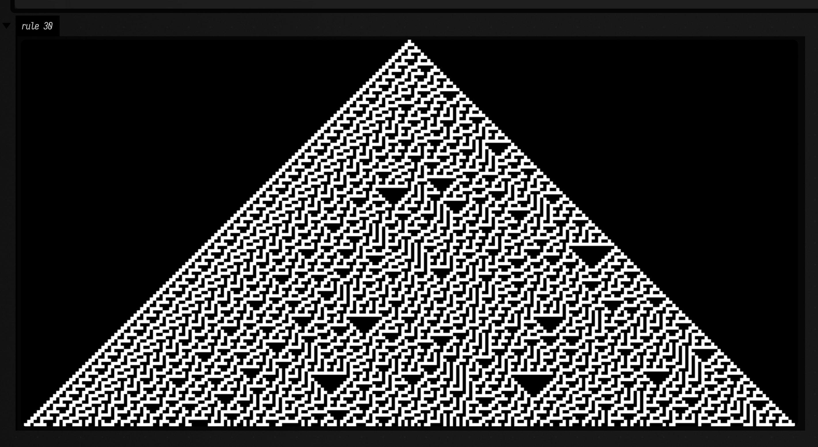
Rule 30 from one live cell, 120 generations. The first 32 cells straight down its middle are one of the two bars below.
Rule 90 and rule 30, as bars
Rule 90 is left XOR right. From a single live cell its space-time diagram is Pascal's triangle
mod 2, which is where the second column of the figure below comes from: binomialParity computes
what row 20 should be from Kummer's theorem, without stepping anything, and
CaSoundDocs.gasketBar compares the real CA
with it cell by cell.
Rule 30's centre column has no such formula.
:::static
// Both derivations run the real stepper. gasketBar additionally checks its row against
// binomialParity before returning, so a wrong answer here throws rather than plays.
val gasket = CaSoundDocs.gasketBar(20)
val chaos = CaSoundDocs.rule30Bar(32)

:::fold the two space-time diagrams, the two bars, and the two notations
/*
Two showImg calls rather than one montage: montage draws its labels into the pixels with a
bitmap font and clips them to the cell, while showImg's `caption` is ordinary text beneath the
image. `toImg(2)` is the STATE COUNT, not a scale: upscaleNearest is what makes a 97-cell row
visible, and passing the upscale to toImg instead dims the live cells to 1/7 grey with no error.
*/
showImg(
    elementaryCa(90, 97, 24).toImg(2).upscaleNearest(9),
    channel = "rule 90",
    maxSide = 1000,
    caption = "rule 90, 24 generations. Row 20, the fourth from the bottom, is the bar.",
)
showImg(
    elementaryCa(30, 67, 32).toImg(2).upscaleNearest(9),
    channel = "rule 30",
    maxSide = 1000,
    caption = "rule 30, 32 generations. The centre column, straight down the middle, is the bar.",
)

showPatRollOf(
    "rule 90 row 20" to gasket.pattern,
    "rule 30 column" to chaos.pattern,
    title = "the two bars, one cycle each",
    subtitle = "${gasket.onsets} of ${gasket.steps} steps against ${chaos.onsets} of ${chaos.steps}",
    cycles = 1,
    channel = "bars",
)

markdown(
    "notation",
    """
| | rule 90, row 20 | rule 30, centre column |
|---|---|---|
| steps | ${gasket.steps} | ${chaos.steps} |
| onsets | ${gasket.onsets} | ${chaos.onsets} |
| shortest notation | `${gasket.condensation.notation}` | `${chaos.condensation.notation}` |
| against a flat spelling | ${gasket.compression.f2} | ${chaos.compression.f2} |
| the search signed for it | ${gasket.condensation.exact} | ${chaos.condensation.exact} |
""",
    width = 1000,
)
:::endfold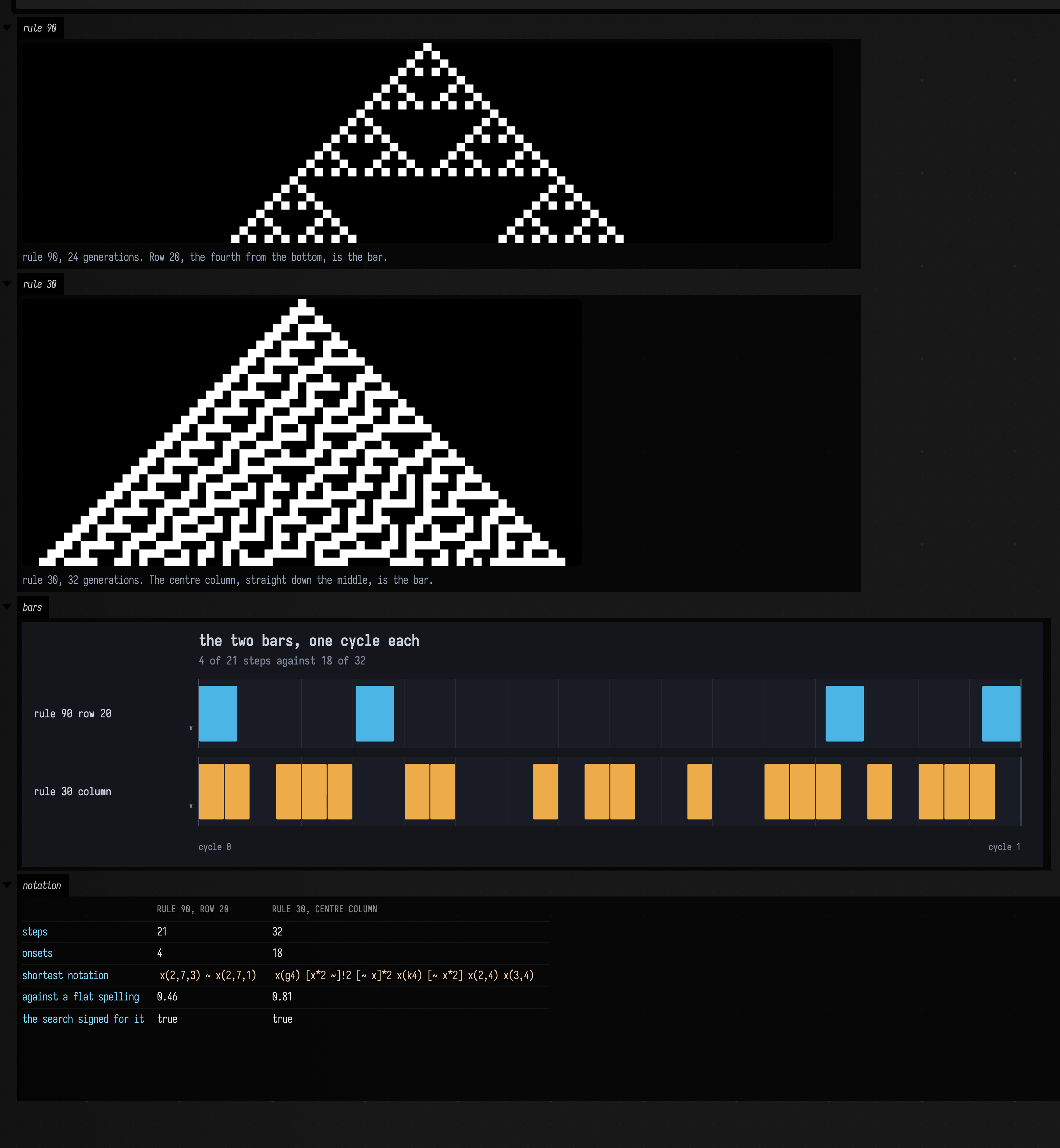
Rule 90's row condenses to two Euclidean figures (x(k,n) spreads k hits as evenly as
possible over n steps; a third number rotates the figure) with a rest between them, and the second is the
first turned: x(2,7) and x(2,7,5) are the same two-in-seven pattern at two rotations. Pascal's
triangle is symmetric in k, so the bar reads the same backwards, and the condenser finds that
symmetry without knowing anything about binomial coefficients.
Rule 30's column condenses as well. A flat spelling carries overhead that any grouping saves, so the number to read is never whether a rhythm compresses but how far, against another rhythm on the same denominator.
Here is the rule-90 bar, four cycles at one cycle per second:
And rule 30's column, three cycles, thirty-two steps each:
The first is a figure you can hum. The second never settles into one, and the two compression numbers measure that difference.
Compression is a ratio of characters, so the atom's length moves it
Both bars above use x as their atom. Spelling the same rhythm with
hh changes the numerator and the denominator by different amounts, and rule 30's 0.83 reads as
0.73 instead. Compare two rhythms only when they are spelled with the same atom.
The same rule read as pitch
Row n of Pascal's triangle mod 2 has exactly 2^popcount(n) odd entries: its population is a
power of two, with the binary digit sum of the generation index as its exponent.
CaSoundDocs.gasketScale counts the real CA's rows and maps that digit sum to a degree of a minor
pentatonic. The tune is the binary expansion of 0, 1, 2, … read out loud: it falls
back to the root at every power of two and climbs through the carries in between.
:::static
/*
gasketPopulations counts the real space-time diagram and throws unless every row's count is
2^popcount(n), so reaching the next line is the check. Plotting the formula as a second trace
would put it exactly under this one and show nothing.
*/
val populations = CaSoundDocs.gasketPopulations()
val notes = CaSoundDocs.gasketScale()

:::fold the populations, and the melody they become
showSignals(
    "live cells per generation" to populations,
    // Short, because a plotly title wider than the plot is clipped rather than wrapped. The
    // claim that this equals 2^popcount(n) is the `check` inside gasketPopulations, not a caption.
    title = "rule 90: live cells per generation",
    xTitle = "generation",
    channel = "populations",
)

showPatRollOf(
    "melody" to pat(notes.joinToString(" ")),
    title = "the same sequence as pitch",
    subtitle = "MIDI ${notes.distinct().sorted().joinToString(", ")} — one degree per binary digit sum",
    cycles = 1,
    pitched = true,
    channel = "melody",
)
:::endfold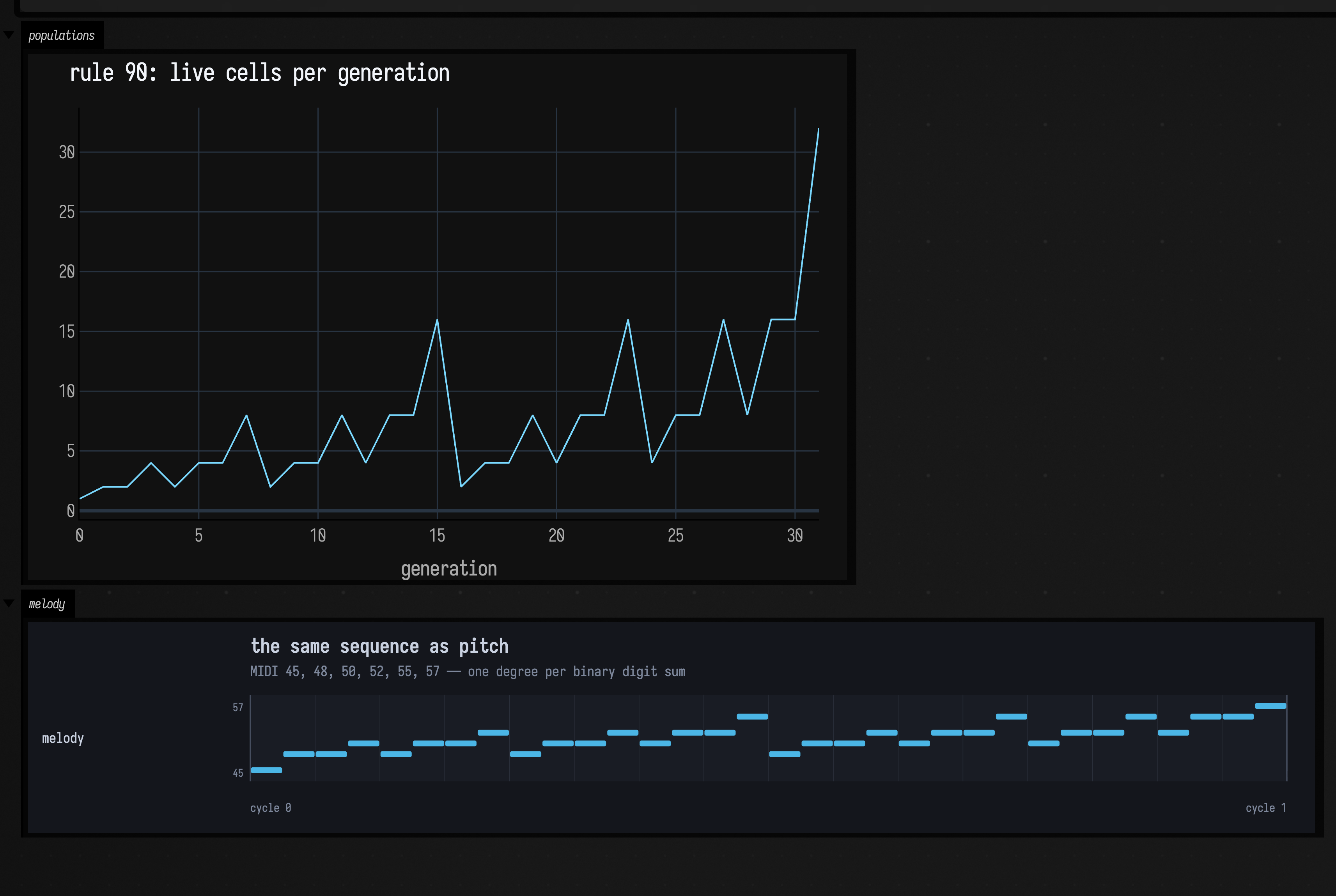
Six rules, one denominator
The same 32-step centre column, taken from six rules, condensed with the same atom. The two clips above are one row of this.
:::static
// The same six rules the harness surveys, so the page and the FIELD_TEST cannot disagree.
val bars = CaSoundDocs.CONDENSATION_SURVEY.map { CaSoundDocs.centreColumnBar(it) }

:::fold lay the six out, worst compression first
val rows =
    CaSoundDocs.CONDENSATION_SURVEY.zip(bars)
        .sortedByDescending { (_, bar) -> bar.compression }
        .joinToString("\n") { (rule, bar) ->
            "| $rule | ${bar.onsets} of ${bar.steps} | ${bar.compression.f2} | " +
                "`${bar.condensation.notation}` |"
        }
markdown(
    "survey",
    """
| elementary rule | onsets | condensed / flat | the shortest notation found |
|---|---|---|---|
$rows
""",
    width = 1080,
)
:::endfold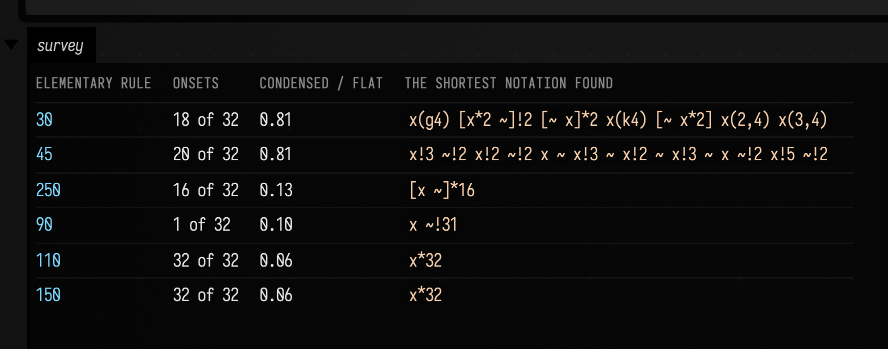
The two rules that resist are the two usually called chaotic. Every other column collapses to a
spelling you could type in one breath: x*32, [x ~]*16, x ~!31. A compressor for music
notation ends up sorting the rules the same way the usual classification does.
The slice matters as much as the rule
Rule 90's centre column compresses to 0.10 and its row 20 to 0.41, and they are the same rule. The column is nearly empty because from one seed only every other cell is ever reachable, so the centre is live only at generation zero. Pick the slice before comparing anything.
Where each piece is documented
- Spatial Artificial Life for the automata: the elementary rules as space-time rasters, Life, cyclic multi-state CA, and the independent oracles the same way this page uses them.
- Patterns & Rhythm for the event model and the mini-notation, and PAT_CONDENSE.md for the condenser.
- Sound and Making a Sound, Every Path There Is for the voice and the other ways to make sound.
- Boolean Network Music Examples is the neighbouring chain: a
different discrete dynamical system, into
NoteProcessand live Dirt triggers rather than into notation.