MorphoHDL in Field
MorphoHDL (Apache-2) is a hardware description language
built on recursive cell division. You write a cell that halves its inputs and calls itself; the
compiler keeps dividing until a SPLIT runs out of bits, and the recursion bottoms out into a
fallback. Bus widths are never declared: a 32-bit adder and an 8-bit adder are the same eleven
lines of source, and the difference is entirely in how far the division ran.
Field runs MorphoHDL's upstream parser, compiler and layout kernel, byte-identical to
commit 3ff923f.
It adds simulation, drawing and an editor; the expansion scheduler is adapted for Field, as
described below.
A morpho box takes upstream's source directly, and a Kotlin box can compile a design with
morphoCircuit(...) in a few lines; both are under Using it, straight after the
pictures.
What it looks like
Four designs out of morpho's standard library, compiled through GraalJS, laid out by morpho's WASM
kernel in 3D, and drawn by Field as vector FLines. Wire colour is signal arrival time: dark
where a value is known early, bright on the critical path. The gradient in each panel is that
circuit's own logic depth. Blue dots are input ports, orange are outputs.
:::static
import afield.lang.morpho.*

/*
Each panel gets its OWN window: these are four different circuits at four different sizes, and a
shared frame would shrink the shifter to a speck to fit the multiplier. Where a shared frame IS
required -- the two adders below, the three projections further down -- it is used and said so.
*/
val designs = [
    Triple("ripple_adder", intArrayOf(16, 16, 1), "carry chain"),
    Triple("brent_kung_adder", intArrayOf(16, 16, 1), "prefix tree"),
    Triple("right_shifter", intArrayOf(32, 5, 1), "mux cascade"),
    Triple("wallace_multiplier", intArrayOf(8, 8), "compression tree"),
]

val panels = designs.map { (design, sig, kind) ->
    val c = morphoCircuit(design, *sig)
    c.growFully(relaxSteps = 220)
    println(
        "%-20s %4d gates  depth %2d  z/xy %.2f  (%s)"
            .format(
                design,
                c.netlist.gateCount,
                c.depth.toInt(),
                c.layout.flatness(),
                kind,
            ),
    )
    "%s(%s) — %d gates, depth %d".format(design, sig.joinToString(","), c.netlist.gateCount, c.depth.toInt()) to
        c.flines(fit = true)
}

// fit = true normalises each panel into the unit square, which is the only way showPlaneGrid can
// frame four differently-sized circuits independently: it takes one window for the whole grid.
showPlaneGrid(
    *panels.toTypedArray(),
    columns = 2,
    cellWidth = 430,
    cellHeight = 430,
    window = morphoUnitWindow(),
)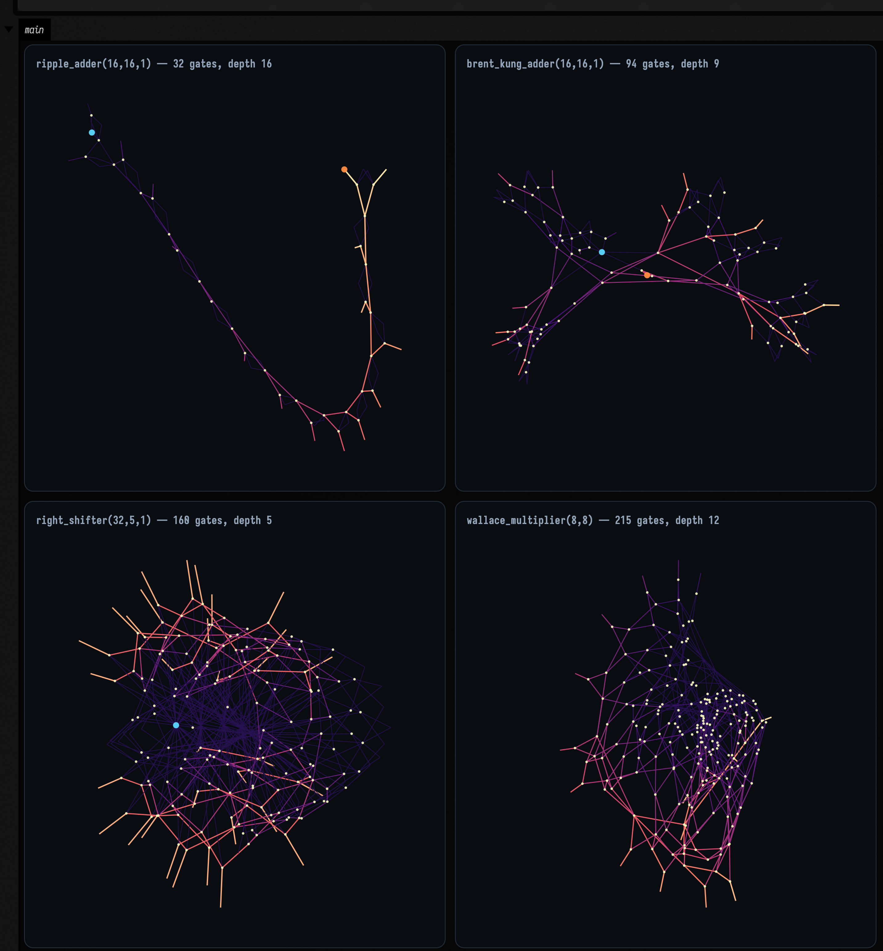
The shapes are the algorithms, up to a point. The ripple adder is a chain because a carry has to walk the whole width, and the Brent–Kung is a branching tree because that is the entire point of a parallel-prefix adder. But a force-directed layout draws connectivity, not a schematic: it will not lay the shifter out as five tidy stages just because it shifts by 1, 2, 4, 8 and 16.
What the shifter shows instead is in the colour. Its 160 gates are nearly all bright, because its depth is 5 and almost everything settles at once. The ripple adder's gates run the whole ramp from dark to bright instead, because a 16-bit carry chain is 16 levels deep. Where the geometry stops being informative, the arrival time takes over.
Using it
As a language
Set a box's main language to MorphoHDL and its children become morpho boxes. A morpho box is MorphoHDL source plus one Field directive:
# main ripple_adder(8, 8, 1)

Xor3 = LUT(3, 0b1001_0110)
Maj3 = LUT(3, 0b1110_1000)

@morpho
def full_adder(a, b, c_in):
    sum = Xor3(a, b, c_in)
    c_out = Maj3(a, b, c_in)
    return sum, c_out

@morpho(fallback=full_adder)
def ripple_adder(a, b, c):
    a0, a1 = SPLIT(a)
    b0, b1 = SPLIT(b)
    s0, c_mid = ripple_adder(a0, b0, c)
    s1, c_out = ripple_adder(a1, b1, c_mid)
    sum = CAT(s0, s1)
    return sum, c_out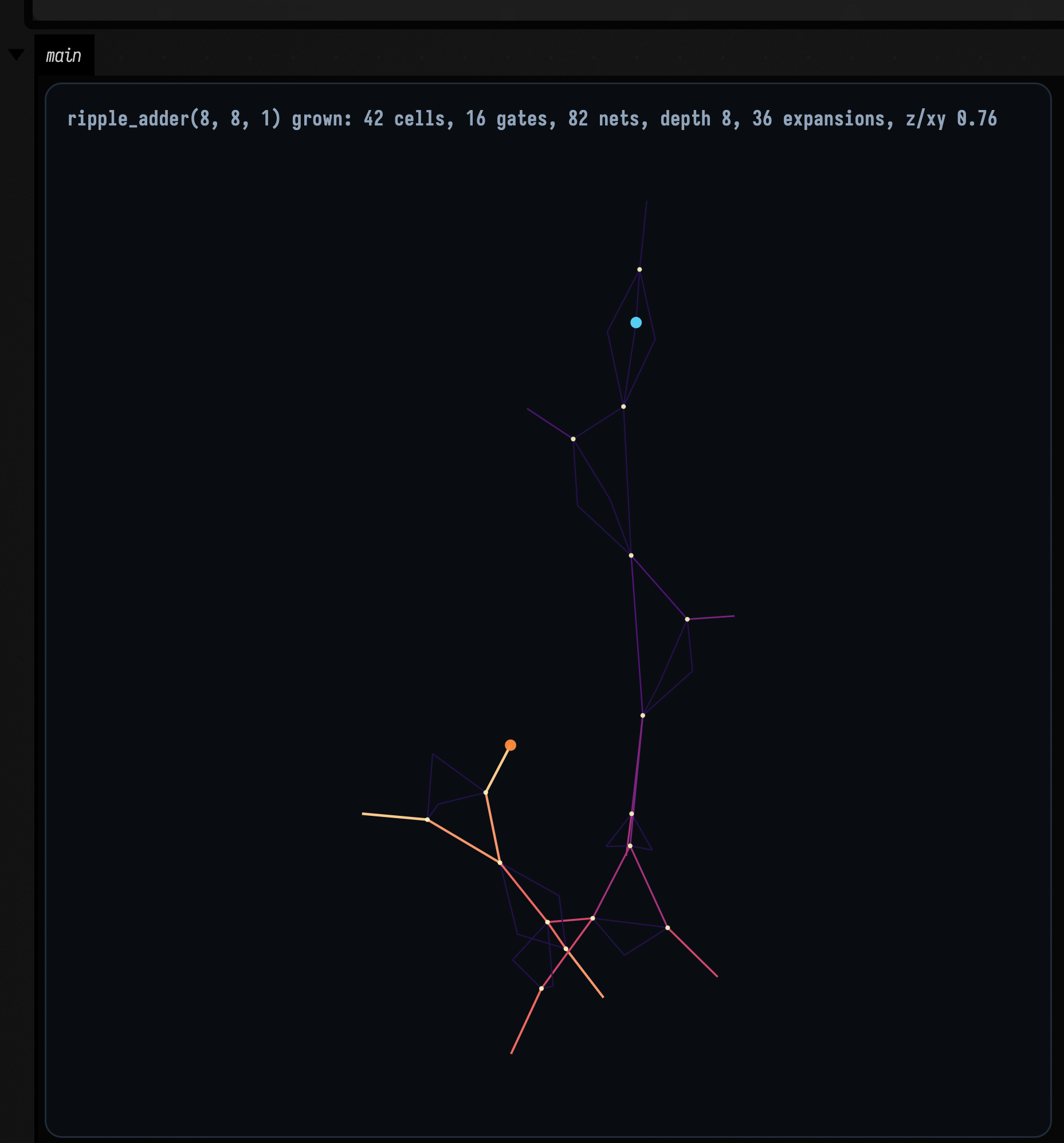
The figure is what that MorphoHDL text produces when the box runs.
The directive is a # comment, which morpho's tokenizer discards, so the same file still parses in
upstream's own tools.
An empty box inherits morpho's standard library. The shortest useful morpho program in Field is one line:
# main brent_kung_adder(32, 32, 1) grow=8 relax=4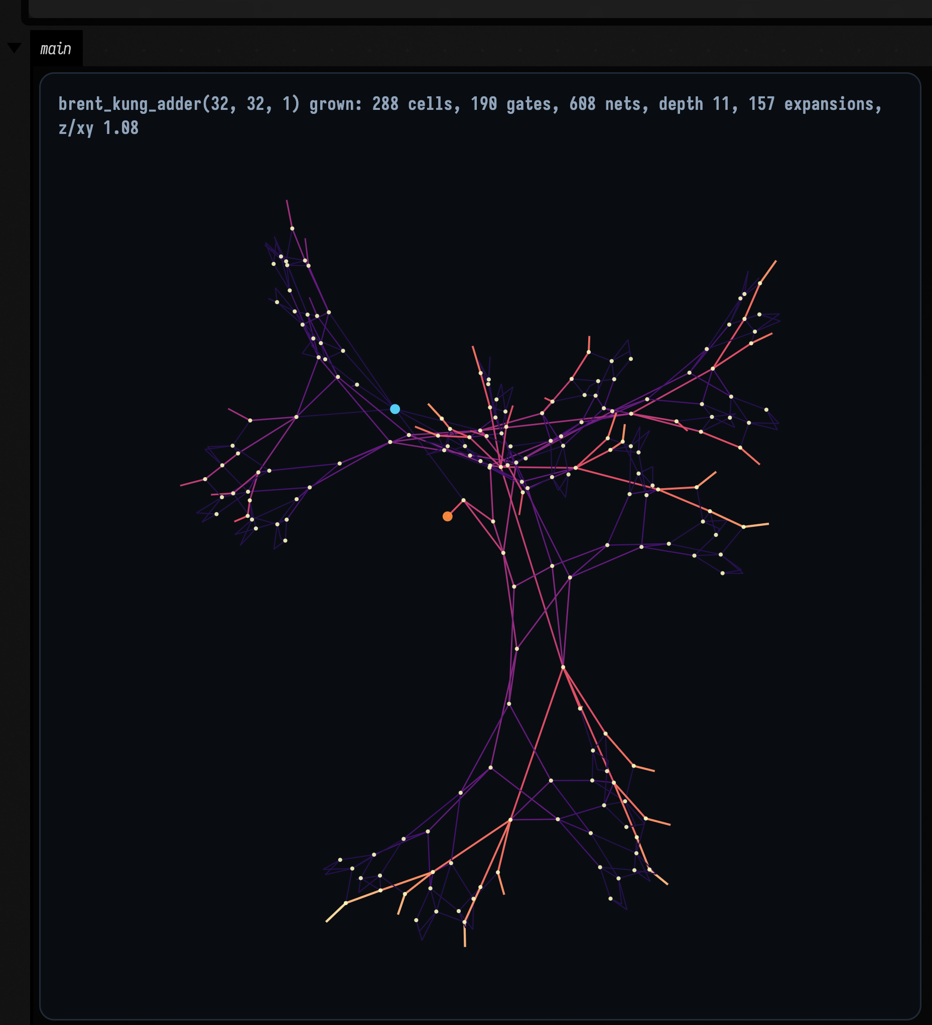
Execute grows the circuit to completion. Launch grows it grow cells per frame and relaxes
the layout relax iterations between expansions, so you can watch the recursion happen.
The directive's widths are required, because a MorphoHDL cell has no width of its own. A box without a directive says so, and lists the cells it found.
From Kotlin
The circuit lands on Box.morphoCircuit. A Kotlin box beside a morpho box can draw it, or skip the
morpho box entirely and compile from Kotlin:
:::static
import afield.lang.morpho.*

val c = morphoCircuit("wallace_multiplier", 16, 16)
c.growFully(relaxSteps = 250)
println(c.summary())

// The simulator is Field's, not morpho's -- there is no logic evaluator in the JavaScript at all.
val a = 48271L
val b = 16807L
val product = c.evaluateOne(a, b)[0]
val check = "%d x %d = %d %s".format(a, b, product, if (product == a * b) "(Kotlin agrees)" else "WRONG")

// Put the check in the panel's title, next to the circuit it is about.
showPlaneGrid(
    "${c.summary()}  |  $check" to c.flines(),
    columns = 1,
    cellWidth = 620,
    cellHeight = 620,
    window = morphoPlaneWindow(c.planeBounds()),
)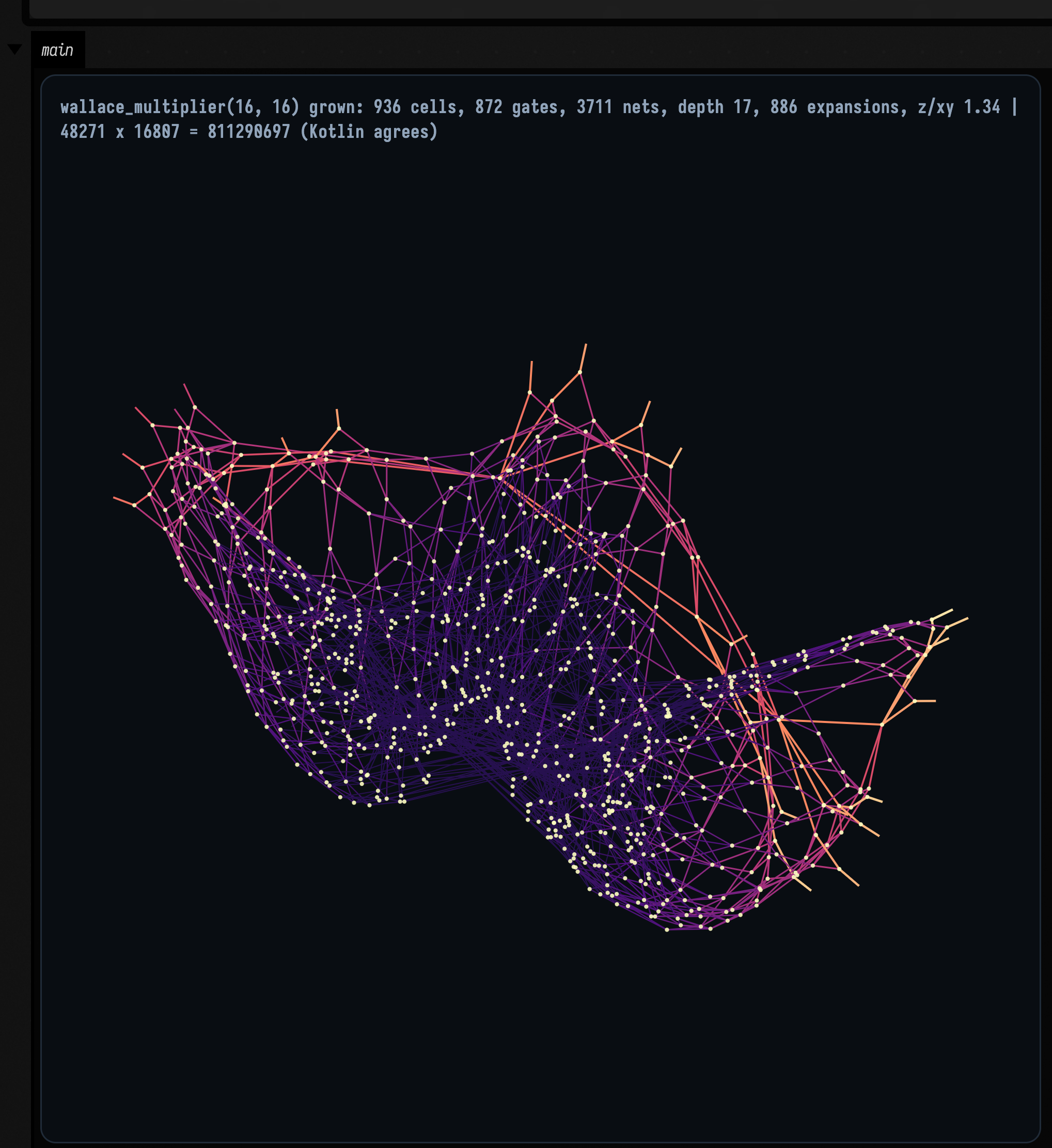
Morpho's compiler produced the netlist, its WASM kernel laid it out, and Field's simulator
multiplied 48271 × 16807 through the gates; the title shows Kotlin's own * agreeing.
flines() gives one FLine per wire and one point-set each for gates, inputs and outputs, coloured
by signal arrival time. Anything Field does with an FLine applies, SVG export and the plane grid
included.
To watch it grow instead:
import afield.lang.morpho.*

val c = morphoCircuit("medusa", 36, 8)
var window: DoubleArray? = null
loop {
    c.step(grow = 24, relax = 6)
    window = morphoWindowUnion(window, c.planeBounds())
    showPlaneGrid(c.summary() to c.flines(), window = morphoPlaneWindow(window!!))
    frame()
}
The projection defaults to isometric, because the layout is 3D. MorphoProjection.XY gives the
view that matches morpho's own renderer.
Which parts of morpho Field runs
MorphoHDL is written in JavaScript, and Field runs it with GraalVM's JS and WASM engines, the same ones its other hosted languages use. Field runs upstream's compiler and layout kernel unchanged and drops upstream's browser rendering:
| upstream file | lines | what it is | in Field? |
|---|---|---|---|
js/parser.js |
216 | tokenizer, parser, SSA | run as-is |
js/primitives.js |
193 | SPLIT/CAT/LSLICE, LUT reduction |
run as-is |
js/compiler.js |
1118 | SoA netlist compiler, width inference, expansion, DCE | run as-is |
js/utils.js |
179 | SoA, MaxHeap, seeded RNG |
run as-is |
graphs_engine/main.wasm |
11 KB | Barnes–Hut force layout | run as-is |
tiny_morpho.py |
867 | Python reference + the MorphoHDL standard library | oracle + stdlib |
js/grower.js |
105 | expansion schedule | reimplemented, 40 lines — see below |
viewer.js, layout_renderer.js, swissgl.js, hex_layout.js, bloom.js, figures.js, demo.js, article.js, presets.js |
~2900 | canvas/WebGL rendering, DOM | dropped |
Field's side of the bridge is in
src/jvmMain/kotlin/afield/lang/morpho/,
and the vendored upstream tree, with a PROVENANCE.md saying what was left out, is under
src/jvmMain/resources/morpho/.
Where this bridge is not upstream's code
grower.js is the exception. Its expansion schedule (largest estimated subtree first, chasing
chains of single-child expansions so a recursion that unrolls one cell at a time does not cost
a frame per level) is what Field wants, but its constructor builds upstream's 2D
LayoutEngine, which Field does not use. The schedule is reproduced in
morpho-field-driver.mjs, and a test compiles a 32-bit Brent–Kung both ways and checks that
the circuits are identical.
Depth: why there are two adders
Morpho's timing pass (updateTimes(),
upstream's own, and what its viewer animates) gives per-cell signal arrival, and the deepest cell
is the critical path.
| width | ripple_adder |
brent_kung_adder |
|---|---|---|
| 4 | 4 | 5 |
| 8 | 8 | 7 |
| 16 | 16 | 9 |
| 32 | 32 | 11 |
| 64 | 64 | 13 |
Drawn at the same width and in the same window (these two are commensurable and are framed together), the difference stops being a table:
:::static
import afield.lang.morpho.*

/*
Same width, same colormap, same window, same everything except the algorithm. Colour is arrival
time normalised PER PANEL, so each shows its own critical path end to end -- the comparison is the
shape of the gradient, not its absolute value, which the depth numbers in the titles carry.
*/
val ripple = morphoCircuit("ripple_adder", 32, 32, 1)
val bk = morphoCircuit("brent_kung_adder", 32, 32, 1)
[ripple, bk].forEach { it.growFully(relaxSteps = 260) }

["ripple_adder" to ripple, "brent_kung_adder" to bk].forEach { (name, c) ->
    println(
        "%-18s %3d gates  depth %2d  %d nets"
            .format(
                name,
                c.netlist.gateCount,
                c.depth.toInt(),
                c.netlist.nNets,
            ),
    )
}

showPlaneGrid(
    "ripple_adder(32,32,1) — 64 gates, depth ${ripple.depth.toInt()}" to ripple.flines(fit = true),
    "brent_kung_adder(32,32,1) — 190 gates, depth ${bk.depth.toInt()}" to bk.flines(fit = true),
    columns = 2,
    cellWidth = 470,
    cellHeight = 470,
    window = morphoUnitWindow(),
)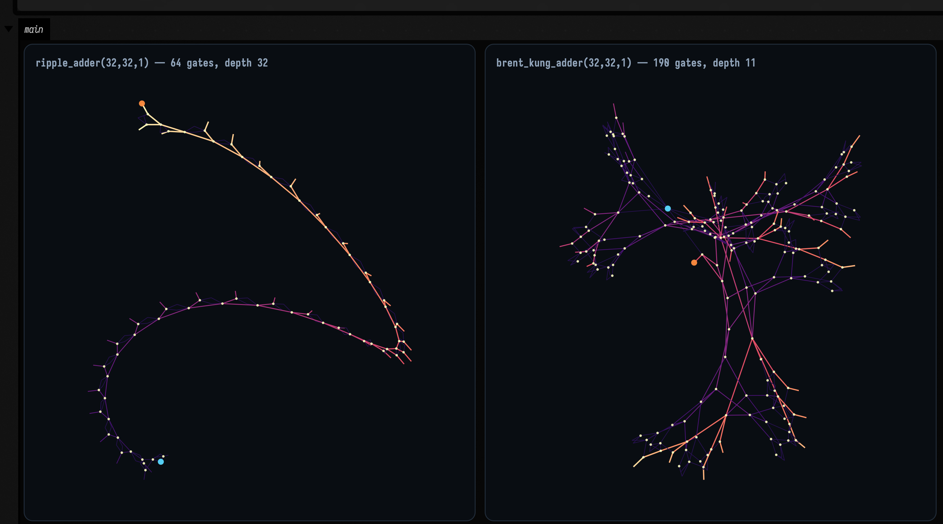
The ripple adder's gradient runs the full length of a single chain — that is the 32 levels. The Brent–Kung reaches its brightest wires after a handful of tree levels and then spends its remaining gates in parallel, which is why it costs three times as many gates (190 against 64) to be three times shallower.
A ripple carry is exactly linear in width. Brent–Kung is \( 2\log_2 N + 1 \). And at four bits the parallel-prefix adder is worse (5 against 4) because its prefix tree costs two levels that a four-stage carry chain never pays for. The crossover is between 4 and 8 bits. That is the real shape of the tradeoff, and measuring it is one line of Kotlin once the language runs inside your environment.
Watching one divide
A language whose only control structure is recursive division should be watched dividing. A morpho
box in launch mode expands a few cells per frame and relaxes the layout between expansions; this
is that loop, recorded straight off a box's output area, one FLine per wire, every frame.
:::static
import afield.lang.morpho.*

// Two designs growing on the same clock. Both start as ONE unexpanded cell -- everything you see
// arrive is morpho's compiler dividing a cell and rewiring what it divided.
val adder = morphoCircuit("brent_kung_adder", 32, 32, 1)
val shell = morphoCircuit("triangle", 32)

// Each panel fits its current geometry into the unit square. As the circuit grows, its scale
// changes too. New cells start at their parent's position before layout relaxation separates them.

loop {
    adder.step(grow = 2, relax = 5)
    shell.step(grow = 12, relax = 5)

    showPlaneGrid(
        "brent_kung_adder — %d gates, %d expansions".format(adder.netlist.gateCount, adder.expansions) to
            adder.flines(fit = true),
        "triangle(32) — %d gates, %d expansions".format(shell.netlist.gateCount, shell.expansions) to
            shell.flines(fit = true),
        columns = 2,
        cellWidth = 470,
        cellHeight = 470,
        window = morphoUnitWindow(),
    )
    frame()
}
Both panels start as a single cell. The adder is given two expansions a frame and the triangle twelve, because they have very different budgets (157 expansions against 993), and matching them would either finish the adder in three seconds or leave the triangle half-built at the end of the clip.
How this clip stays vector
Field's other animated figures are rasters by construction: animateEvolution's panels lambda
is typed List<Pair<String, Img>>, and a clip built that way is pixels before it is ever
recorded. This one is not. The docs runner's record-box is a Playwright recording of the box's
output element — a launched box that calls showPlaneGrid every frame is recorded with
every frame drawn as real SVG. The mp4 is an encoding of vector frames rather than a montage of
bitmaps, which is why the wires stay hairline-thin as the circuit fills the panel.
Circuits laid out in three dimensions
Morpho's layout kernel, graphs_engine/main.wasm, is a 3D Barnes–Hut force solver, and Field runs
it as it is. Upstream's browser driver, force_layout.js, flattens every particle onto a plane on
every frame:
this.pos[p * 3 + 2] = 0.0;
this.vel[p * 3 + 2] = 0.0;
Field's driver leaves z free, so the circuits come out as solids. MorphoLayout.flatness() reports
the z extent over the larger of the x and y extents; a value near 1 means the circuit is as deep as
it is wide.
Three views of one circuit, sharing a window. The only thing that differs between the panels is where the camera is:
:::static
import afield.lang.morpho.*

/*
One circuit, one layout, three cameras. XY is the view morpho's own renderer is restricted to,
because force_layout.js pins z. XZ looks straight down the axis XY drops: if the layout really
were planar, THAT panel would be a horizontal line and nothing else.
*/
val c = morphoCircuit("brent_kung_adder", 32, 32, 1)
c.growFully(relaxSteps = 300)

val b = c.layout.bounds()
println("extent  x %.1f  y %.1f  z %.1f".format(b[3] - b[0], b[4] - b[1], b[5] - b[2]))
println("z / max(x,y) = %.2f".format(c.layout.flatness()))

showPlaneGrid(
    "XY — what morpho's own renderer sees" to c.flines(projection = MorphoProjection.XY, fit = true),
    "XZ — down the axis XY discards" to c.flines(projection = MorphoProjection.XZ, fit = true),
    "isometric" to c.flines(projection = MorphoProjection.ISOMETRIC, fit = true),
    columns = 3,
    cellWidth = 340,
    cellHeight = 340,
    window = morphoUnitWindow(),
)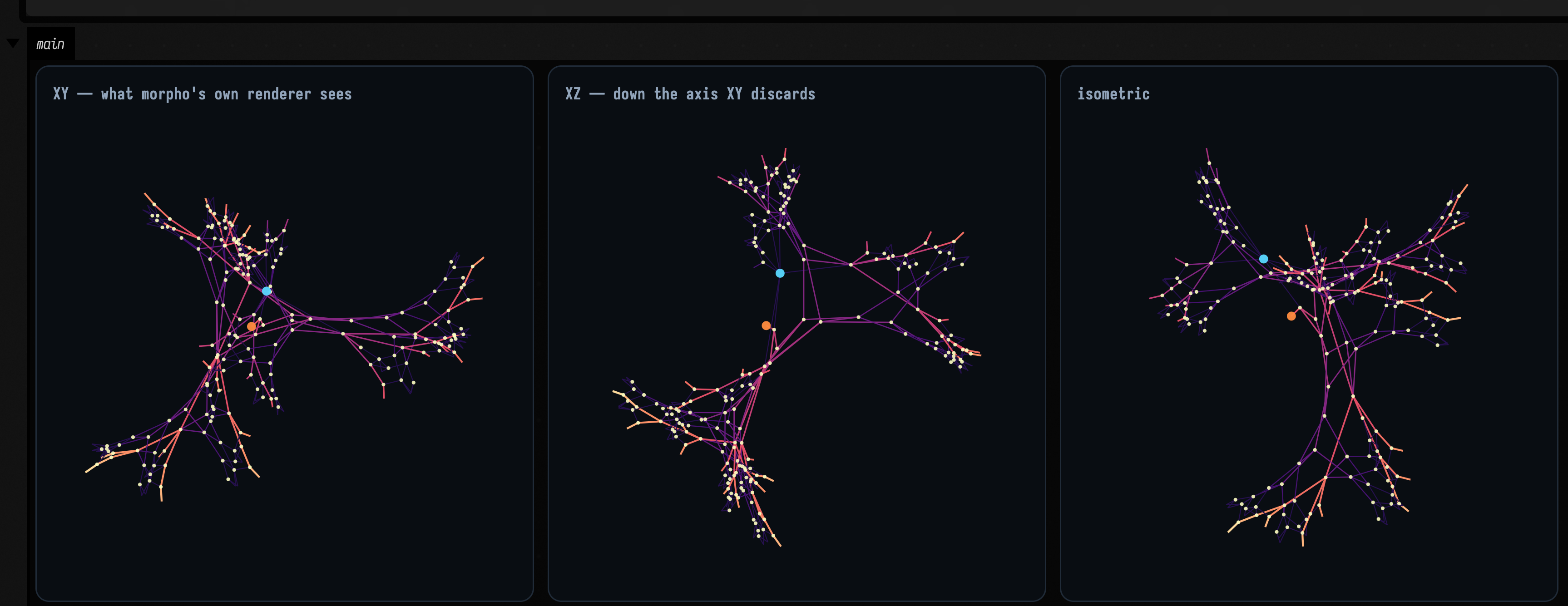
The middle panel does the work here. It is the view along the axis the flat renderer throws away, and if the layout were planar it would be a single horizontal line. It is not.
The clip below orbits the same circuit, so no single angle is doing the work. It is fully grown and completely static; only the azimuth changes.
:::static
import afield.lang.morpho.*

// NOTHING about the circuit changes in this clip -- it is grown before the loop starts and never
// stepped again. Every frame re-projects the same fixed 3D positions from a new angle.
val c = morphoCircuit("brent_kung_adder", 32, 32, 1)
c.growFully(relaxSteps = 320)

// One window covering every azimuth, so the circuit turns instead of breathing. Recomputing the
// frame per angle would rescale it on every frame and hide the very thing being demonstrated.
var window: DoubleArray? = null
for (i in 0 until 48) {
    window = morphoWindowUnion(window, c.planeBounds(morphoOrbit(i * Math.PI / 24.0), padFraction = 0.06))
}
val viewWindow = morphoPlaneWindow(window!!)

var azimuth = 0.0
loop {
    azimuth += 0.026
    showPlaneGrid(
        "brent_kung_adder(32,32,1) — %d gates, azimuth %3d°"
            .format(
                c.netlist.gateCount,
                Math.round(Math.toDegrees(azimuth)) % 360,
            ) to c.flines(projection = morphoOrbit(azimuth)),
        columns = 1,
        cellWidth = 700,
        cellHeight = 700,
        window = viewWindow,
    )
    frame()
}
A flat layout would collapse to a line twice per turn. This one does not, at any angle.
Whether the circuits are right
The compiled circuits are checked two ways. Field simulates them against integer arithmetic,
exhaustively for the 8-bit ripple adder, where a wiring mistake would show only on the rare input
whose carry runs the full width. And their gate counts match morpho's separate Python
implementation, tiny_morpho.py, gate for gate on the adders, the multiplier and the shifter.
What a circuit costs to compile and simulate
The largest design here, a 4 144-gate medusa(36,8), compiles and fully expands in about 270 ms
once Graal has warmed up; a 32-bit Brent–Kung adder takes about 50 ms. Relaxing the layout 200 steps
costs between about 20 ms and 1.5 s depending on size, and you rarely want it in one go —
step(grow, relax) in a loop spreads it over frames.
Simulation is bit-parallel: each net holds a Long whose bit s is that net's value for sample
s, so one LUT evaluation covers 64 inputs at once, and the exhaustive 8-bit adder check takes a
fraction of a second.
See also
- Searching for MorphoHDL circuits: generating MorphoHDL programs from a specification, with random sampling, hill climbing and a population, and what they find.
- Rewriting Your Own Syntax and Language Extensions for making a syntax of your own and teaching the editor about it.
- How this bridge to a foreign runtime was built, step by step, is in
dev_docs/MORPHO_LANGUAGE_BRIDGE.md, for anyone hosting another language.