Proving a Function's Range

A plot of a function is a set of samples joined up. Anything narrower than the gap between two samples can fall between them, and the plot gives no sign that it did. For most work that's fine. When you need to know that a control signal never goes above 0.9, or where its real peak is, sampling more densely only makes a miss less likely.

Functions.Fn can answer those questions with interval arithmetic. Instead of evaluating f(x) at a number, Field evaluates it over a whole interval [a, b] at once and gets back a range [lo, hi] that every value of f on that interval is guaranteed to lie inside. The enclosure covers values between plot samples too. Splitting the interval and evaluating each half can tighten the bounds; the search reports whether it reached the requested tolerance within its work budget.

A bump the plot misses

Here is a sawtooth with a very narrow gaussian bump added to it: half a millisecond wide, on a six-second window. Sampled at 1,200 points, the samples are 5 ms apart, so they step straight over it.

:::static
val f = with(Functions) {
    saw(0.7, amplitude = 0.4) + gaussian(2.31, 0.0005, 0.6, Functions.Domain.ALL)
}

// What a plot sees: the largest of 1200 samples.
val sampled = (0 until 1200).maxOf { f.eval(6.0 * it / 1199) }

// One enclosure of the whole window: sound, but loose.
val once = f.enclose(0.0, 6.0)

// Branch-and-bound: the real maximum, with the x that reaches it.
val range = f.certifiedRange(0.0, 6.0)

// A yes/no question with the same guarantee.
val claim = f.certifiedNeverExceeds(0.42, 0.0, 6.0)

display(
    "answers",
    Table(["question", "answer"], title = "saw + a 0.5 ms bump on [0, 6]")
        .row("largest of 1200 samples", sampled)
        .row("f.enclose(0, 6)", "[${once.lo}, ${once.hi}]")
        .row("certifiedRange: max reached", "${range.max!!.value} at x = ${range.max!!.witness}")
        .row("certifiedRange: max proven ≤", range.max!!.bound)
        .row("certifiedNeverExceeds(0.42)", "${claim.kind} at x = ${claim.witness}"),
)

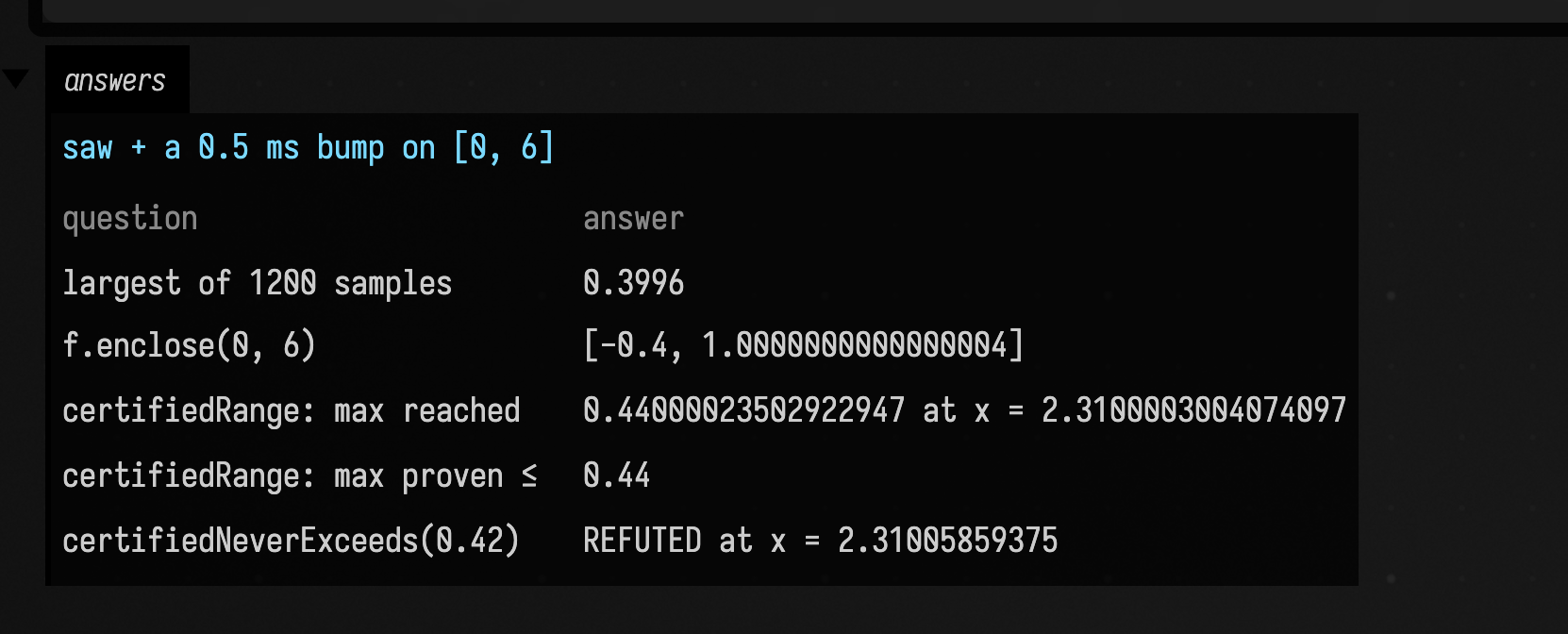
The samples say the function peaks at 0.4. The single enclosure says the peak is no higher than about 1.0, which is true but not useful. certifiedRange finds the bump at x = 2.31 and pins its height between a value it actually computed there and a bound it proved, less than a millionth apart. certifiedNeverExceeds(0.42) is refuted, and the result carries the x that breaks the claim.

The three calls:

• f.enclose(a, b) is one interval evaluation. It's cheap, and always correct, but it can be much wider than the true range.
• f.certifiedRange(a, b, tolerance) keeps splitting the interval, always refining the piece that could still hold a better extreme, until the value it reached and the bound it proved are within tolerance.
• certifiedNeverExceeds, certifiedNeverBelow, certifiedEquals and certifiedReaches answer a claim with PROVEN, REFUTED (with a witness x) or UNDECIDED if the work budget ran out.

There is also f.certifiedEnvelope(a, b, bins), which gives a proven [lo, hi] for each of bins equal slices. The signal viewer draws it as a band behind a channel made with certifiedSignalChannel(...).

Seeing the proof

showIntervals(f, a, b) runs certifiedRange on both extremes, records every interval the search evaluated, and draws them:

:::static
val f = with(Functions) {
    saw(0.7, amplitude = 0.4) + gaussian(2.31, 0.0005, 0.6, Functions.Domain.ALL)
}
showIntervals(f, 0.0, 6.0, title = "saw + a 0.5 ms bump")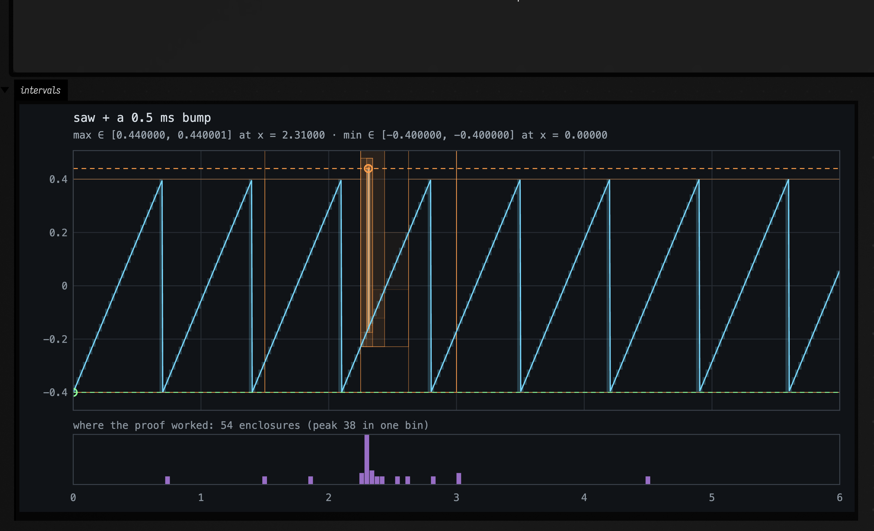

Reading it from back to front:

• Boxes. Each rectangle is one interval evaluation: over its x span, every value of f lies within its height. Orange boxes belong to the search for the maximum, green to the minimum. A box drawn strongly was split further; a faint one was dropped because its bound couldn't beat the best value already found.
• Band. The blue band is the certified envelope. Where the sampled line drops at each saw reset, the band covers the jump. At this width the band is tight enough to sit almost on the line; the narrow orange boxes around x = 2.31 are where the search closed in on the bump.
• Line. The sampled curve: what an ordinary plot would draw.
• Dots and dashed rules. The witness (the best value actually computed) and the proven bound for each extreme.

The purple strip underneath counts evaluations per slice of x. Nearly all of the maximum's work happens in one slice, around the bump. The minimum takes almost no work, because the saw's lowest value, -0.4, is reached exactly at x = 0.

f.intervalPicture(a, b) returns the same picture without displaying it, so it can be the last expression of a box or go into display(...) yourself.

The waveform generators

saw, triangle and square can be bounded like any other formula op. Each one takes the fractional part of (x - phase) / period, and that is the case plain interval arithmetic handles worst. Over a hundred periods, t runs from 0 to 100, so t - floor(t) taken as two separate numbers comes out as [-100, 100]. Field recognises the t - floor(t) shape and bounds it as one value: exact inside a single period, [0, 1] across a boundary.

The triangle needs one more step. Its shape is if (t < 0.5) 2t else 2 - 2t. When the interval straddles 0.5, both branches are possible, and bounding each branch over all of t gives [0, 2] for each, so the triangle comes out as [-1, 3]. Instead, each branch is bounded knowing the comparison that chose it: 2t only for t below 0.5, 2 - 2t only for t at or above it.

:::static
val cases = with(Functions) {
    [
        "saw(0.5)" to saw(0.5),
        "triangle(0.5)" to triangle(0.5),
        "square(0.5, duty = 0.3)" to square(0.5, duty = 0.3),
        "saw + square * triangle" to (saw(1.0) + square(0.25) * triangle(2.0)),
        "pulseTrain, jittered" to
            pulseTrain(
                c(0.5, Functions.Domain.ALL),
                duty = c(0.4, Functions.Domain.ALL),
                rise = c(0.05, Functions.Domain.ALL),
                jitter = c(0.3, Functions.Domain.ALL),
                domain = Functions.Domain.ALL,
            ),
        "saw, eased BOUNCE_OUT" to saw(1.0, amplitude = 0.5, offset = 0.5).ease(Functions.Easing.BOUNCE_OUT),
        "valueNoise(1, 3)" to valueNoise(1L, 3.0),
        "fn { x -> x * x }" to fn(0.0..100.0, "lambda") { x -> x * x },
    ]
}
val table = Table(
    ["function", "one enclosure on [-17.3, 83.9]", "refused because"],
    title = "One-shot bounds across about two hundred periods",
)
for ((name, f) in cases) {
    val e = f.enclose(-17.3, 83.9)
    table.row(name, if (e.certified) "[${e.lo}, ${e.hi}]" else "-", e.refusal ?: "")
}
display("oscillators", table)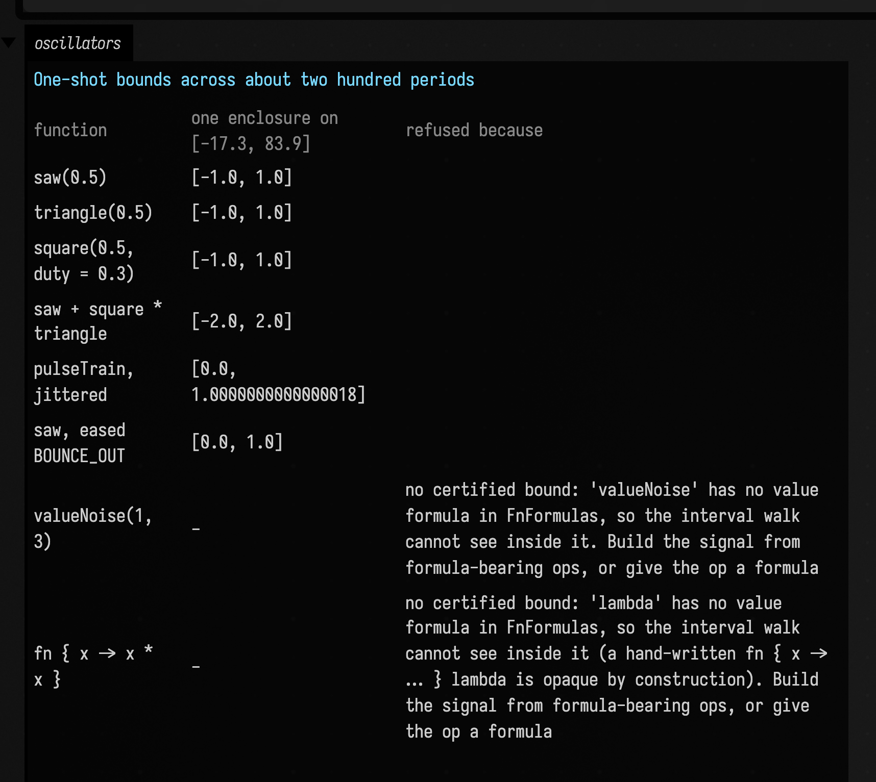

One enclosure over two hundred periods gives each generator its exact amplitude, or a few ulps more for the jittered pulse train, whose phase arithmetic rounds more often.

pulseTrain and the easings (ease, tween) are bounded too. Their formula depends on settings stored on the node (which edge shape, which body profile, which easing), so Field builds a formula for each combination it meets. A jittered pulse train moves each cycle by a seeded hash of the cycle number. Over a piece of x that spans only a few cycles, that hash is bounded by computing it for each of them; over more, it is anywhere in [0, 1].

The last two rows are refused, and refusal is the only thing Field does with a function it can't bound. A bound it guessed would look exactly like one it proved.

What can be bounded

Anything built from ops that have a formula: arithmetic, sin and cos, the three generators above, gaussian, ramp, remap, smoothStep, pulseTrain, ease and tween with any of their settings, step, sign, abs, floor, exp, log, pow, atan2, hypot, clamp, softClip, the windows, the modulators (amplitudeMod, ringMod) and the x-transforms (shift, warp, scaleX). A formula is also what gives an op an exact gradient for fitGradient, so the two lists are almost the same.

Refused, by name:

• Lambdas (fn { ... }, mapX, mapY): there is only compiled code, and nothing to read a formula from.
• Noise (valueNoise, perlinNoise, fbm, ...): the value is a hash of position.
• pulseBurst and pulsePattern: built on pulseTrain, with their own record of which pulses sound.
• Ops that carry data (piecewise, splines, timeline, sequence, ...).

FnIntervals.unsupportedOps(f) lists what stops a given function from being bounded.