Mapper graphs of point clouds

A cloud of points has a shape: it can be one blob or several, a strand, a tree with branches, a ring. Mapper draws that shape as a small graph. Every point gets a lens value, a number saying something about where it is. The range of the lens is cut into overlapping bins, the points in each bin are grouped into clusters, every cluster becomes a node, and clusters that share points are joined. Branches, loops and separate pieces of the cloud come out as branches, loops and separate pieces of the graph.

This example scatters points along a ring with a tail, plus a separate blob, colours each point by its lens (here eccentricity, how far it is on average from all the others) and draws the Mapper graph over them, each node at the middle of its cluster and sized by how many points it holds:

import afield.geometry.topology.mapper.*

// A ring with a tail, and a separate blob, 1500 points in all.
val random = java.util.Random(4)
val points = DoubleArray(1500 * 2)
for (i in 0 until 1500) {
    val (x, y) = when {
        i < 800 -> {
            val t = random.nextDouble() * 2 * PI
            80 + 45 * cos(t) to 85 + 45 * sin(t)
        }
        i < 1150 -> {
            val s = random.nextDouble()
            112 + 70 * s to 117 + 40 * s
        }
        else -> 160 + 12 * random.nextGaussian() to 35 + 12 * random.nextGaussian()
    }
    points[2 * i] = x + 2.5 * random.nextGaussian()
    points[2 * i + 1] = y + 2.5 * random.nextGaussian()
}

val graph = Mapper.compute(points, lens = Mapper.eccentricity(points), intervals = 12, overlap = 0.35)
val black = Img(200, 170, 3, FloatArray(200 * 170 * 3))
showImgGrid(
    "${graph.components().size} pieces, ${graph.loops} loop(s)" to
        black.drawFLines([graph.pointsFLine(pointSize = 1.5)] + graph.toFLines(), scale = 3.0),
    columns = 1,
    cellSide = 600,
)

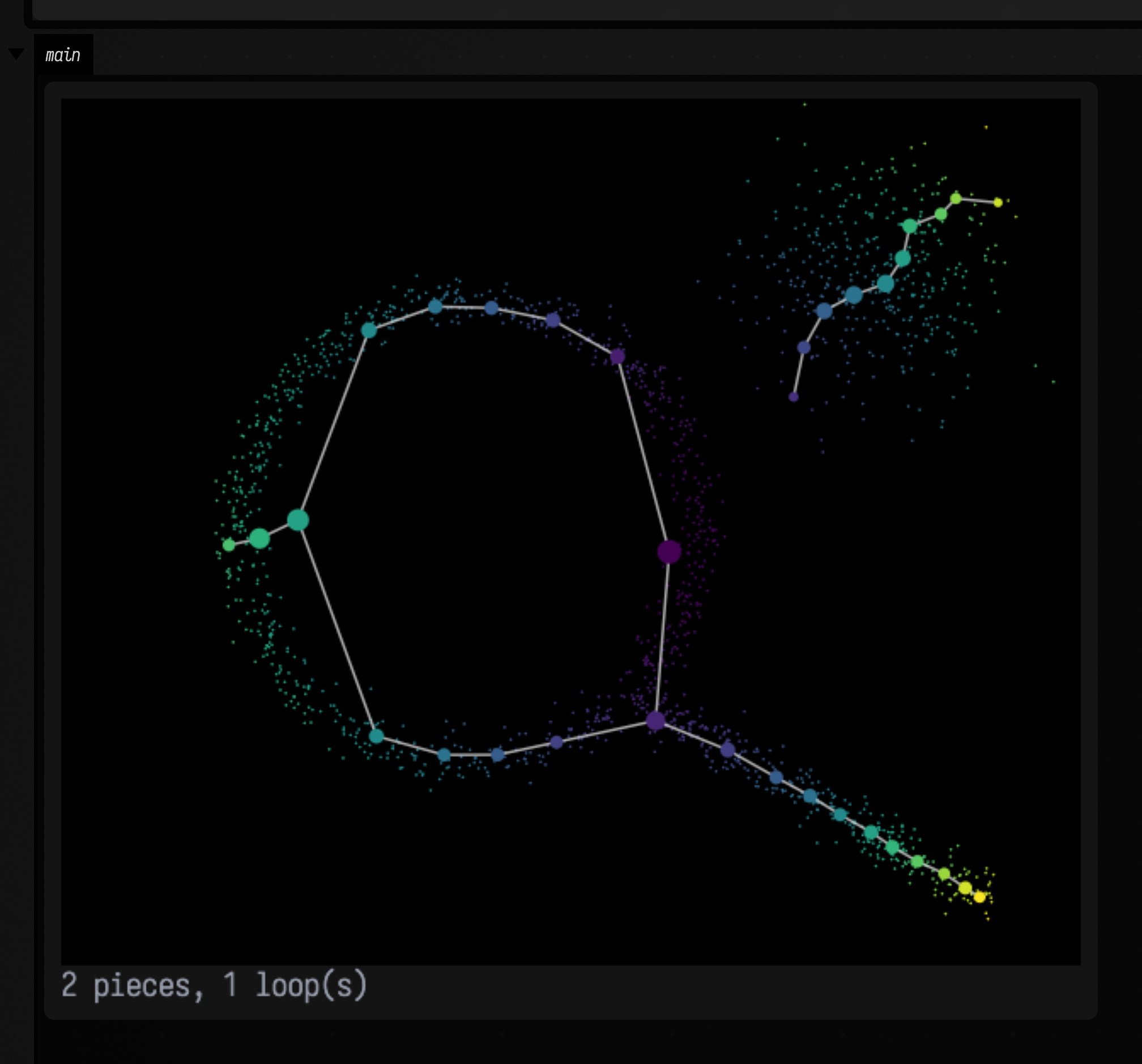
on black, a cloud of small dots coloured from dark purple in the middle to yellow at the extremities: a ring with a tail running off to the lower right, and a separate round blob at the upper right. Over them, a graph of grey lines and larger coloured dots follows the same shapes: a loop of nodes around the ring, a chain along the tail, and a short chain on the blob

The caption counts what the graph found: the components (pieces) and the loops. The ring is one loop. The tail ends in a node with one neighbour, and the blob is a piece on its own. The blob comes out as a chain rather than a single node because eccentricity changes across it: its near side is closer to everything else than its far side.

Choosing the lens

The lens decides what the graph is sensitive to. Branches and loops show up only when the lens varies along them; a lens that is constant across a ring folds it into a line.

Mapper.coordinate(points, axis = 0) slices the cloud along one axis, like a CT scanner. It is simple and predictable, but blind to structure running across the slices.
Mapper.eccentricity(points) is small in the middle of the cloud and large at its extremities, so branch ends stand out whichever way they point. It is the usual first choice for finding branches.
Mapper.density(points, k) is high where points crowd together, so it separates dense cores from sparse fringes. Sparse fringes can split into many small clusters.
Any DoubleArray with one value per point works: time, a measured quantity, a distance from some landmark.

This example draws the graph of the same cloud through each of the three lenses:

import afield.geometry.topology.mapper.*

val random = java.util.Random(4)
val points = DoubleArray(1500 * 2)
for (i in 0 until 1500) {
    val (x, y) = when {
        i < 800 -> {
            val t = random.nextDouble() * 2 * PI
            80 + 45 * cos(t) to 85 + 45 * sin(t)
        }
        i < 1150 -> {
            val s = random.nextDouble()
            112 + 70 * s to 117 + 40 * s
        }
        else -> 160 + 12 * random.nextGaussian() to 35 + 12 * random.nextGaussian()
    }
    points[2 * i] = x + 2.5 * random.nextGaussian()
    points[2 * i + 1] = y + 2.5 * random.nextGaussian()
}

val black = Img(200, 170, 3, FloatArray(200 * 170 * 3))
fun panel(name: String, lens: DoubleArray): Pair<String, Img> {
    val graph = Mapper.compute(points, lens = lens, intervals = 12, overlap = 0.35)
    return "$name: ${graph.loops} loop(s)" to
        black.drawFLines([graph.pointsFLine(pointSize = 1.5)] + graph.toFLines(), scale = 2.0)
}
showImgGrid(
    panel("x", Mapper.coordinate(points, axis = 0)),
    panel("eccentricity", Mapper.eccentricity(points)),
    panel("density", Mapper.density(points, k = 10)),
    columns = 3,
    cellSide = 300,
)

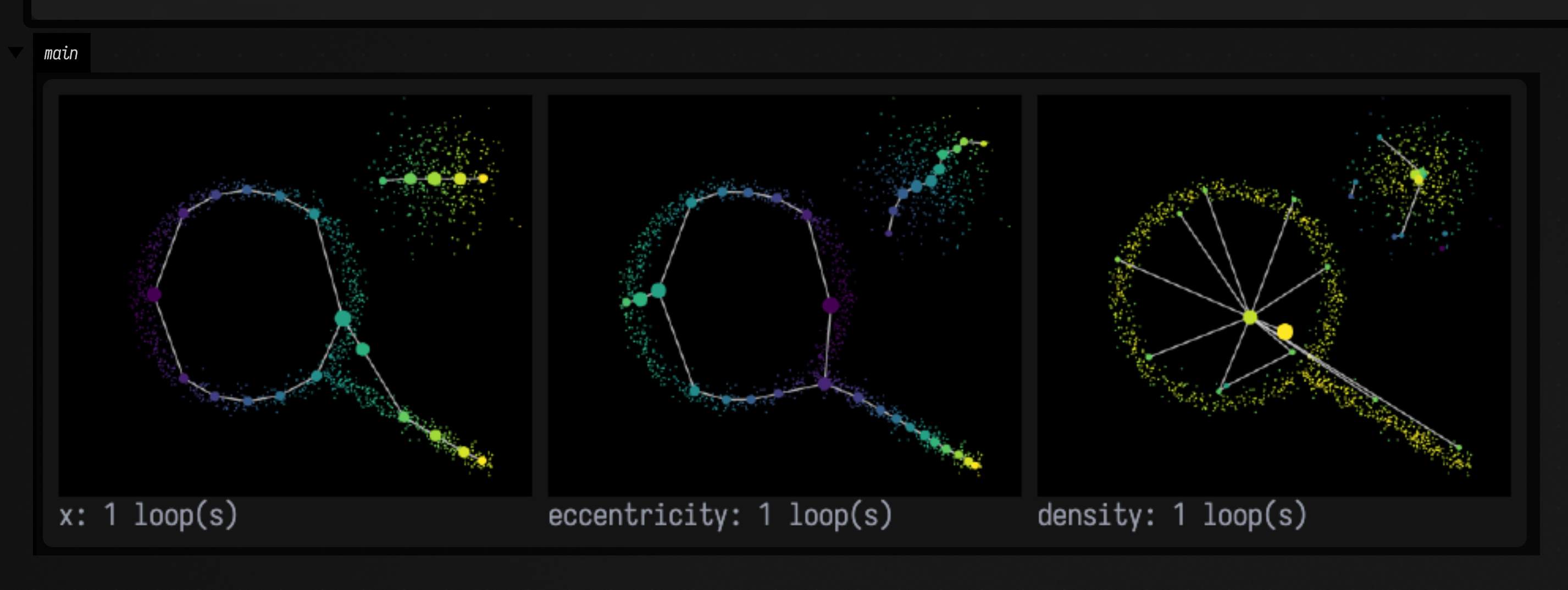
The x and eccentricity lenses both vary along the ring, and both graphs look like the cloud. The density lens is nearly the same all the way round the ring, so the whole ring lands in one or two bins, and the centre of a cluster that is a whole ring is the middle of the hole. When a Mapper graph stops looking like the cloud, try another lens and compare what it reveals.

The other settings are intervals (how many bins: more gives a finer graph), overlap (the fraction each bin shares with the next: more joins clusters more readily), eps (the largest gap inside one cluster, by default three times the median distance from a point to its eighth nearest neighbour) and minClusterSize (smaller clusters are dropped as noise).

Loops and branches in strokes

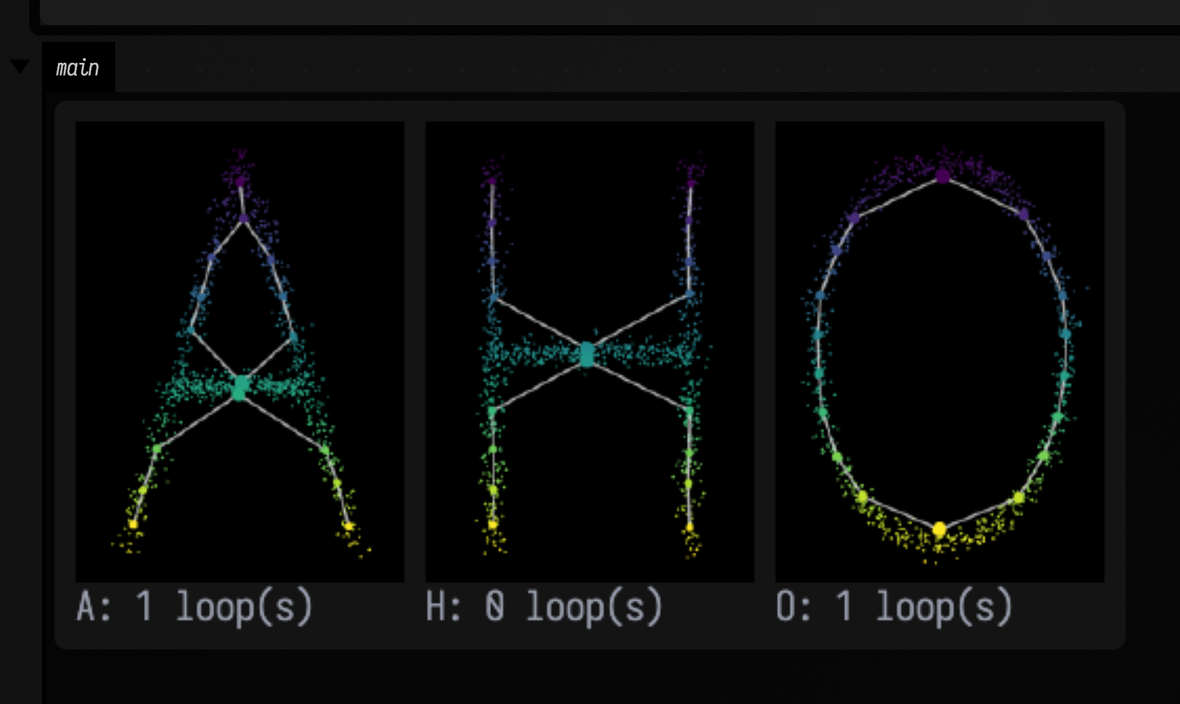
Strokes are point clouds too. This example scatters points along three letters and uses the vertical coordinate as the lens, so each bin is a horizontal slice. An A splits into two legs below its apex and is joined across by its bar, which closes a loop. An H is two posts joined once, a tree. An O is a loop.

import afield.geometry.topology.mapper.*

// Each letter as straight strokes (x0, y0, x1, y1) in a 100 by 140 box; O is a circle.
val strokes = mapOf(
    "A" to [[50.0, 10.0, 15.0, 130.0], [50.0, 10.0, 85.0, 130.0], [30.0, 80.0, 70.0, 80.0]],
    "H" to [[20.0, 10.0, 20.0, 130.0], [80.0, 10.0, 80.0, 130.0], [20.0, 70.0, 80.0, 70.0]],
)
val random = java.util.Random(2)
fun letter(name: String): DoubleArray {
    val out = DoubleArray(900 * 2)
    for (i in 0 until 900) {
        val s = random.nextDouble()
        val (x, y) = if (name == "O") {
            val t = s * 2 * PI
            50 + 38 * cos(t) to 70 + 58 * sin(t)
        } else strokes.getValue(name)[i % 3].let { (x0, y0, x1, y1) -> x0 + s * (x1 - x0) to y0 + s * (y1 - y0) }
        out[2 * i] = x + 2.0 * random.nextGaussian()
        out[2 * i + 1] = y + 2.0 * random.nextGaussian()
    }
    return out
}

val black = Img(100, 140, 3, FloatArray(100 * 140 * 3))
showImgGrid(
    *["A", "H", "O"]
        .map { name ->
            val points = letter(name)
            val graph =
                Mapper.compute(points, lens = Mapper.coordinate(points, axis = 1), intervals = 10, overlap = 0.35)
            "$name: ${graph.loops} loop(s)" to
                black.drawFLines(
                    [graph.pointsFLine(pointSize = 1.5)] + graph.toFLines(minSize = 3.0, maxSize = 9.0),
                    scale = 2.0,
                )
        }
        .toTypedArray(),
    columns = 3,
    cellSide = 220,
)

three panels on black, each a letter made of scattered dots coloured from purple at the top to yellow at the bottom, with its Mapper graph over it: the A's graph runs down from the apex, splits into two legs and closes a loop through the bar; the H's graph is two vertical chains joined in the middle; the O's graph is a ring. The captions read A: 1 loop(s), H: 0 loop(s), O: 1 loop(s)

Mapper and principal curves answer the same question in different ways. Mapper is quick, works in any number of dimensions, and reports topology (pieces, branches and loops) without fitting anything, but its nodes sit at cluster centres and its edges are straight. Principal curves fit smooth curves through the middle of the points, with widths, at the cost of an optimisation. A Mapper graph is a good way to decide how many curves, and whether to allow branches, before fitting.

What you get

A MapperGraph has nodes (each a MapperNode with its members, the point indices; its centroid, lens and bin; and size) and edges (each a MapperEdge between nodes a and b, with how many points they shared). components() lists the connected pieces, loops counts independent loops, and nodesOfPoint says which nodes each point belongs to.

toFLines() draws the graph over the first two coordinates, pointsFLine() draws the points coloured by lens, and network() returns the graph as a GeometryNetwork with the nodes' size and lens as channels. Points can also be a List<Vec2>, and 3D or higher-dimensional points work with dimension.