Signal examples: time and frequency

Signal processing needs pictures. A filter can reveal structure or erase the detail you cared about. An event detector can catch a gesture or promote a random spike. The first two examples here work sample by sample in the time domain and keep the raw stream and the processed stream in the same frame; the rest of the page asks what a signal is made of, in frequency.

Filter chains as layered curves

Stacking three filters is easy; seeing whether the stack helped is not. What you want from a smoothing chain is less junk and the same gesture, and those two are traded against each other.

:::static
val raw = mutableListOf<Float>()
val smooth = mutableListOf<Float>()
val filtered = mutableListOf<Float>()

val ema = EMAFilter(alpha = 0.08f)
val oneEuro = OneEuroFilter(minCutoff = 1.0f, beta = 0.02f, sampleRate = 120f)
val band = BandPassFilter(frequency = 5f, sampleRate = 120f, q = 0.8f)

for (i in 0 until 420) {
    val t = i / 120f
    val signal =
        (sin(2.0 * PI * 1.2 * t).toFloat() * 0.7f +
            sin(2.0 * PI * 4.7 * t + 0.3).toFloat() * 0.22f +
            (-0.12f + random().toFloat() * 0.24f))
    raw += signal
    val s = oneEuro(ema(signal))
    smooth += s
    filtered += band(s)
}

// One call puts all three streams on one axis — raw, the smoothed chain, and the band-passed
// component each get their own trace (dark theme + cyan/orange palette applied).
showSignals(
    "raw" to raw,
    "EMA + One-Euro (smoothed)" to smooth,
    "band-pass (5 Hz)" to filtered,
    channel = "main",
    xTitle = "sample",
)

One showSignals call puts all three streams on one axis. Watch the chain order: band is applied to s, the output of ema and oneEuro, not to signal, so the band-pass sees a stream the two smoothers have already been through.

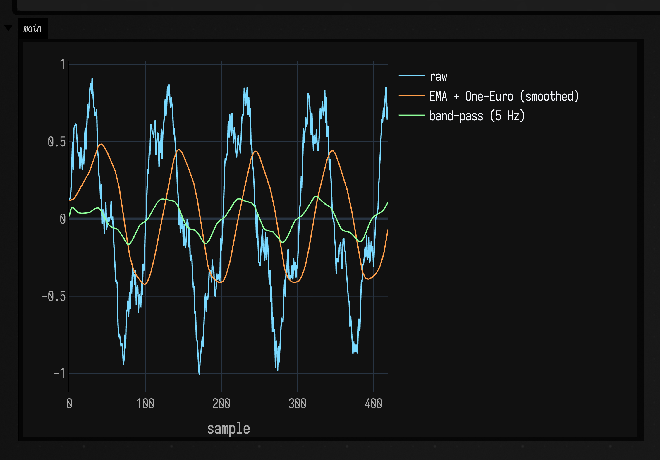
That order is why the band-pass trace is small and slow: the smoothers upstream removed most of the 4.7 Hz content it is tuned for, so what gets through is a little of the slower 1.2 Hz swing. BandPassFilter and OneEuroFilter both take sampleRate = 120f, so their cutoffs in Hz are right for stored data pushed through in a loop.

Distribution-aware event flags

Event detectors answer a different question from the filters above: did something noteworthy happen? Both of these fit a distribution to the last windowSize samples and fire when the newest one lands in a tail, so nothing fires at all until the window has filled: 64 samples of the 360 here.

:::static
val gammaEvents = GammaEventDetector(windowSize = 64, tailProbabilityThreshold = 0.03f, influence = 0.15f)
val betaEvents = BetaEventDetector(
    windowSize = 64,
    supportMin = -1f,
    supportMax = 1f,
    lowerTailThreshold = 0.04f,
    upperTailThreshold = 0.04f,
)

val raw = mutableListOf<Float>()
val eg = mutableListOf<Float>()
val eb = mutableListOf<Float>()

for (i in 0 until 360) {
    val t = i / 120f
    var x = (sin(2.0 * PI * 1.1 * t) * 0.55 + (-0.08 + random() * 0.16)).toFloat()
    if (i % 83 == 0) x += 0.95f
    if (i % 127 == 0) x -= 0.8f
    raw += x
    eg += gammaEvents(kotlin.math.abs(x))
    eb += betaEvents(x)
}

// The raw stream and both detectors' verdicts on one axis — the event traces flag their tail
// crossings (beta fires either way, ±1) over the raw motion, so which departures triggered is clear.
showSignals(
    "raw" to raw,
    "gamma events" to eg,
    "beta events" to eb,
    channel = "main",
    xTitle = "sample",
)

The stream gets a +0.95 spike at every 83rd sample and a -0.8 dip at every 127th, and both detectors report their verdict on the same axis as the signal: 1f from the gamma detector on the sample that fired, and from the beta detector +1f for an upper-tail event and -1f for a lower-tail one.

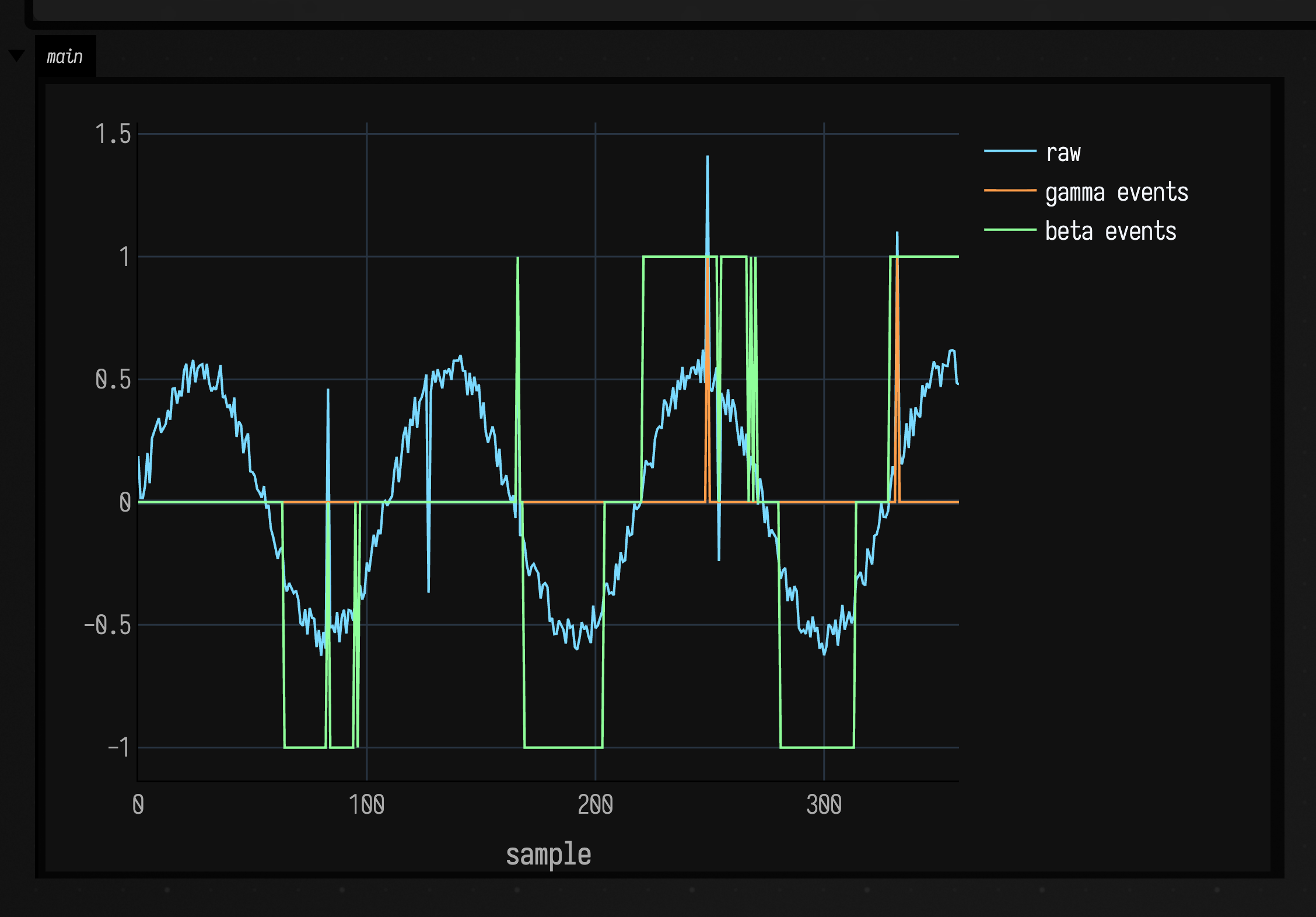
The gamma detector, fed abs(x), marks single samples. The beta detector holds +1 and -1 across whole stretches instead, and its window is why: 64 samples is shorter than the 109 the 1.1 Hz sine takes to come round at 120 samples a second, so every fit is a fit over a trend and the trend's own continuation keeps landing in a tail. Give a distribution fit at least one full cycle of any periodic component, or detrend before the detector sees it.

For inline diagnostics of similar live values, continue with Visualizers. When you need to estimate a state you can only measure indirectly, see State estimation.

From time to frequency

Sometimes the question is what a signal is made of: which frequencies carry the energy, how bright the timbre is, where a chirp is heading. For that Field has an FFT, a windowed Spectrum, a Spectrogram (a short-time FFT, or STFT), the usual spectral features, and a resonator bank, which measures energy at frequencies you choose without running a transform at all. Any length of signal can be transformed, not just powers of two, and nothing needs an external library or a GPU.

Each example below synthesises its own signal, analyses it, and draws the result into the box's output.

One spectrum

Synthesise a rising chirp plus two steady tones, run a Hann-windowed FFT, and read the shape back out. fft(...) returns a Spectrum that knows its sample rate, so bins map to real Hz and the feature helpers return frequencies you can label.

:::static
// Synthesise a rising linear chirp + two steady tones, FFT it, draw the one-sided spectrum.
val sampleRate = 8000.0
val n = 2048
val f0 = 300.0
val f1 = 3000.0
val dur = n / sampleRate
val k = (f1 - f0) / dur
val signal =
    DoubleArray(n) { i ->
        val t = i / sampleRate
        // Rising linear chirp (phase-integrated so instantaneous freq sweeps cleanly) + two tones.
        0.9 * sin(2.0 * PI * (f0 * t + 0.5 * k * t * t)) +
            0.4 * sin(2.0 * PI * 700.0 * t) +
            0.3 * sin(2.0 * PI * 1800.0 * t)
    }

val spec = fft(signal, WindowType.HANN, sampleRate)
val mag = spec.magnitudeOneSided() // bins 0 .. N/2
val freqs = spec.frequencies() // bin -> Hz
val centroid = spec.centroid() // magnitude-weighted mean frequency, Hz
val rolloff = spec.rolloff(0.85) // freq below which 85% of the energy sits
val peak = spec.peakFrequency() // dominant component, Hz

// One call puts the magnitude curve on screen against real Hz, with the centroid and 85% rolloff
// marked as dashed reference lines. showSignals(...) applies the dark theme + cyan/orange palette.
showSignals(
    "magnitude" to mag.toList(),
    x = freqs.toList(),
    channel = "main",
    xTitle = "frequency (Hz)",
    yTitle = "magnitude",
    marks = [
        "centroid ${centroid.f0} Hz" to centroid,
        "85% rolloff ${rolloff.f0} Hz" to rolloff,
    ],
)
println(
    "peak=${peak.f0}Hz centroid=${centroid.f0}Hz rolloff=${rolloff.f0}Hz bins=${mag.size}",
)

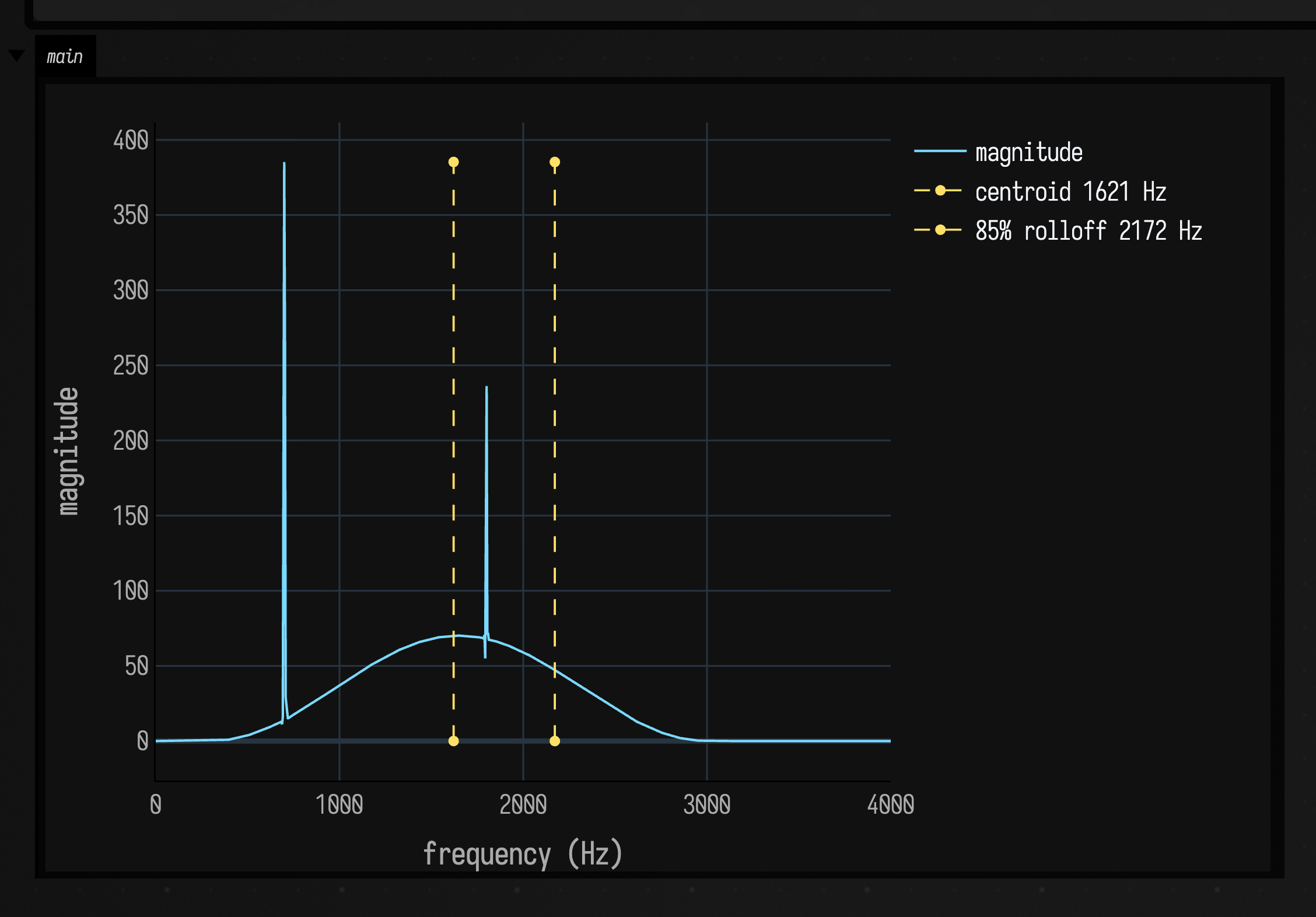
The tall spike is the steady 700 Hz tone, the broad hump is the chirp's energy spread across the frequencies it swept, and the dashed lines mark the spectral centroid and the 85% rolloff.

A spectrogram of a chirp

A single spectrum is one slice. An STFT frames the signal, windows each frame, hops forward, and transforms — giving you a spectrogram: a time × frequency heatmap. The rising chirp becomes a diagonal ridge, the steady tones stay as horizontal lines, and the per-frame spectral centroid draws a bright trace climbing with the chirp. showHeatmap(...) draws the [frame][bin] matrix through a colormap, low frequencies at the bottom, into the box's output.

:::static
// --- signal: a rising linear chirp (300 -> 3000 Hz) plus two steady tones (700, 1800 Hz) ---
val sampleRate = 8000.0
val n = 24000 // 3 s
val f0 = 300.0
val f1 = 3000.0
val dur = n / sampleRate
val k = (f1 - f0) / dur
val signal =
    DoubleArray(n) { i ->
        val t = i / sampleRate
        // Phase-integrated chirp so the instantaneous frequency f0 + k*t sweeps cleanly below Nyquist.
        0.9 * sin(2.0 * PI * (f0 * t + 0.5 * k * t * t)) +
            0.35 * sin(2.0 * PI * 700.0 * t) +
            0.30 * sin(2.0 * PI * 1800.0 * t)
    }

// --- STFT -> magnitude heatmap + spectral-centroid trace ---
val spec = stft(signal, fftSize = 1024, hopSize = 256, window = WindowType.HANN, sampleRate = sampleRate)
val mags = spec.magnitudes() // [frame][bin]
val maxMag = spec.maxMagnitude().coerceAtLeast(1e-9)
val centroid = spec.centroidTrace() // Hz per frame
val nyquist = sampleRate / 2.0

// dB relative to the peak (a useful dynamic range), as a [frame][bin] matrix.
val dB =
    Array(spec.numFrames) { f ->
        DoubleArray(spec.numBins) { b -> 20.0 * log10((mags[f][b] / maxMag).coerceAtLeast(1e-4)) }
    }
// The spectral centroid as a normalized (x, y) overlay: x = time fraction, y = fraction of Nyquist.
val trace =
    centroid.indices.map { f ->
        (f.toDouble() / (spec.numFrames - 1).coerceAtLeast(1)) to (centroid[f] / nyquist).coerceIn(0.0, 1.0)
    }

println(
    "frames=${spec.numFrames} bins=${spec.numBins} centroid ${centroid.first().f0} -> ${centroid.last().f0} Hz",
)
// One showHeatmap call: transpose [frame][bin] to time × frequency, low frequency at the bottom
// (flipY), the house cyan→orange ramp over a [-80, 0] dB range, with the centroid as a bright overlay.
showHeatmap(
    dB,
    colormap = "cyanorange",
    width = 1800,
    height = 840,
    vmin = -80.0,
    vmax = 0.0,
    transpose = true,
    flipY = true,
    overlay = trace,
    overlayThickness = 3,
)

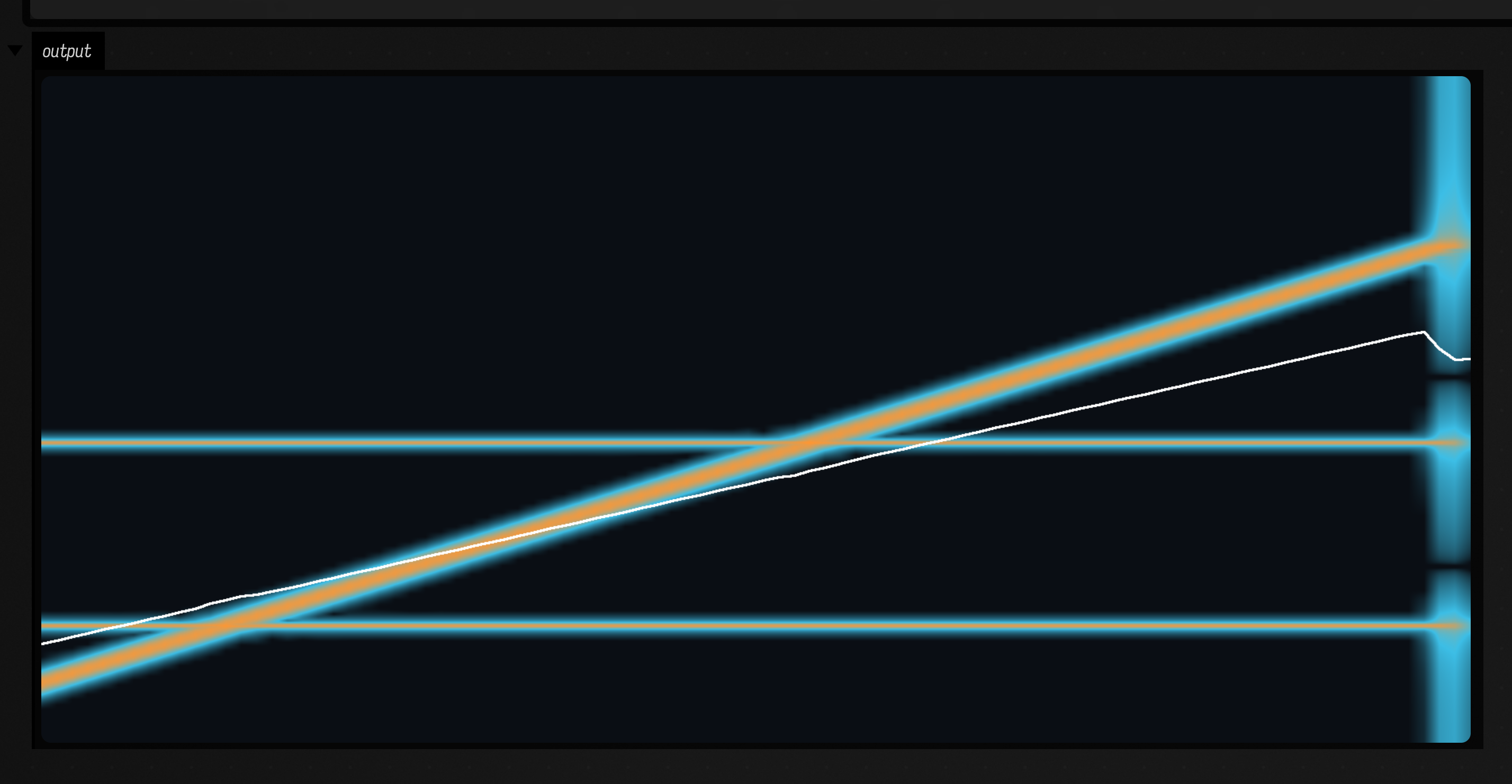
The diagonal ridge is the chirp, the two flat lines are the 700 Hz and 1800 Hz tones, and the thin trace is the centroid climbing with the sweep. The STFT produces the [frame][bin] magnitudes; one showHeatmap call renders them (cyan→orange over a [-80, 0] dB range) and draws the centroid overlay.

Mel bands — a perceptual, log-frequency view

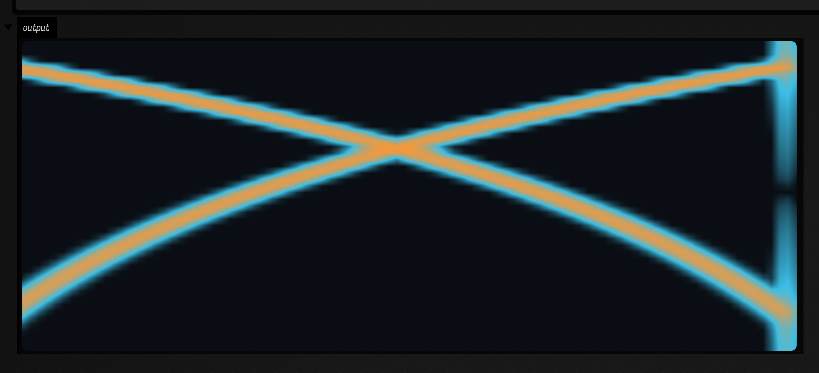
An FFT's bins are evenly spaced in Hz, so most of them land in the upper octaves, where a fixed number of Hz is a smaller and smaller musical interval. The mel scale warps frequency logarithmically; Mel.filterBank(...) collapses a magnitude spectrum into a handful of triangular mel bands. Applied per STFT frame it gives a mel-spectrogram. Here the signal is two crossing chirps — one rising, one falling — so they trace an X, curved by the log warping.

:::static
// --- signal: two crossing chirps, one rising (200 -> 3200 Hz) and one falling (3200 -> 200 Hz) ---
val sampleRate = 8000.0
val n = 24000
val up0 = 200.0
val up1 = 3200.0
val dn0 = 3200.0
val dn1 = 200.0
val dur = n / sampleRate
val ku = (up1 - up0) / dur
val kd = (dn1 - dn0) / dur
val signal =
    DoubleArray(n) { i ->
        val t = i / sampleRate
        0.7 * sin(2.0 * PI * (up0 * t + 0.5 * ku * t * t)) + 0.7 * sin(2.0 * PI * (dn0 * t + 0.5 * kd * t * t))
    }

// --- STFT -> per-frame mel filter bank -> heatmap ---
val spec = stft(signal, fftSize = 1024, hopSize = 256, window = WindowType.HANN, sampleRate = sampleRate)
val numBands = 48
val mel = Array(spec.numFrames) { Mel.filterBank(spec.magnitude(it), sampleRate, numBands, 0.0, sampleRate / 2.0) }
var maxMel = 1e-9
for (row in mel) for (v in row) if (v > maxMel) maxMel = v

// dB relative to the peak, as a [frame][band] matrix.
val dB =
    Array(spec.numFrames) { f ->
        DoubleArray(numBands) { b -> 20.0 * log10((mel[f][b] / maxMel).coerceAtLeast(1e-4)) }
    }

println("frames=${spec.numFrames} bands=$numBands")
// transpose [frame][band] to time × mel-band, low band at the bottom.
showHeatmap(
    dB,
    colormap = "cyanorange",
    width = 1800,
    height = 720,
    vmin = -80.0,
    vmax = 0.0,
    transpose = true,
    flipY = true,
)

A resonator bank — frequency analysis without a transform

An FFT frames the signal and asks all frequencies at once, on a fixed linear grid set by the transform size. A resonator bank turns that around: run the signal through a set of complex one-pole resonators, each tuned to a frequency you pick, and each resonator's running magnitude is the energy near its frequency. There is no window and no frame blocking; it is a per-sample IIR filterbank, so it streams. Choosing the frequencies yourself also means you can space them logarithmically (like the ear) and give each its own time constant. resonate(...) runs a fixed bank offline and hands back the per-hop complex output; resonatorAlphaHeuristics(...) computes a smoothing coefficient per frequency, so high resonators settle faster than low ones.

:::static
import afield.audio.engine.resonate
import afield.audio.engine.resonatorAlphaHeuristics

// --- same rising chirp (300 -> 3000 Hz) + two tones (700, 1800 Hz), as a Float signal ---
val sampleRate = 8000f
val n = 24000
val f0 = 300.0
val f1 = 3000.0
val durS = n / sampleRate.toDouble()
val k = (f1 - f0) / durS
val signal =
    FloatArray(n) { i ->
        val t = i / sampleRate.toDouble()
        (0.9 * sin(2.0 * PI * (f0 * t + 0.5 * k * t * t)) +
                0.35 * sin(2.0 * PI * 700.0 * t) +
                0.30 * sin(2.0 * PI * 1800.0 * t))
            .toFloat()
    }

// --- a bank of complex resonators, log-spaced from 120 Hz to 3900 Hz ---
val numRes = 96
val minHz = 120.0
val maxHz = 3900.0
val freqs =
    FloatArray(numRes) { i ->
        kotlin.math.exp(ln(minHz) + (ln(maxHz) - ln(minHz)) * i / (numRes - 1)).toFloat()
    }
val alphas = resonatorAlphaHeuristics(freqs, sampleRate) // per-frequency smoothing / time constant
val hop = 256

// resonate returns, per hop slice: numRes real parts then numRes imag parts.
val flat = resonate(signal, sampleRate, freqs, alphas, betas = alphas, hopLength = hop)
val slices = flat.size / (2 * numRes)
fun ampAt(s: Int, kk: Int): Float {
    val base = s * 2 * numRes
    val re = flat[base + kk]
    val im = flat[base + numRes + kk]
    return kotlin.math.sqrt(re * re + im * im)
}
var maxA = 1e-9f
for (s in 0 until slices) for (kk in 0 until numRes) {
    val a = ampAt(s, kk)
    if (a > maxA) maxA = a
}

// dB relative to the peak, as a [slice][resonator] matrix.
val dB =
    Array(slices) { s ->
        DoubleArray(numRes) { kk -> 20.0 * log10((ampAt(s, kk).toDouble() / maxA).coerceAtLeast(1e-4)) }
    }

println("resonators=$numRes slices=$slices freq ${freqs.first().toInt()} -> ${freqs.last().toInt()} Hz")
// transpose [slice][resonator] to time × resonator, low (low-Hz) resonator at the bottom.
showHeatmap(
    dB,
    colormap = "cyanorange",
    width = 1800,
    height = 720,
    vmin = -80.0,
    vmax = 0.0,
    transpose = true,
    flipY = true,
)

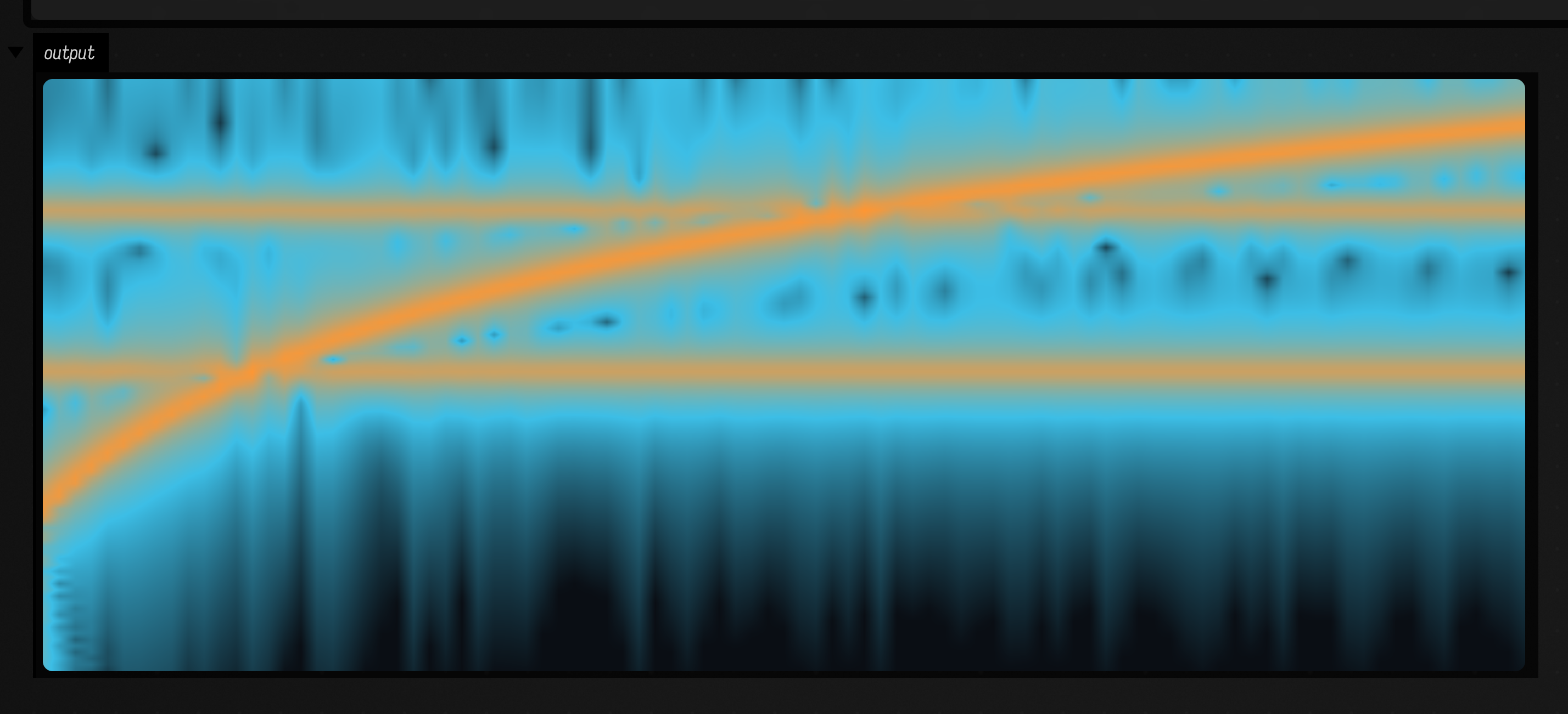
Same chirp ridge and two tone lines as the STFT view, but now on a log-frequency axis (the tones sit closer together up top) and with each band carrying its own time constant instead of one shared window. Because the bank is recursive and per-sample it also runs live as a streaming analyzer. TrackingResonatorBank goes further: each resonator estimates the phase drift of its own output and retunes towards the instantaneous frequency whenever its local power clears a dynamic threshold, falling back to its natural frequency when the partial goes away.

Streaming features that compose with the filter chain

The spectral features also come as FloatFilters, so they slot straight into the same then chain as the time-domain filters. Feed one sample in, get the latest feature out (held between hops). Here a rising chirp plus a couple of onsets drives three features at once, and the three traces are drawn stacked in the box's output.

:::static
// --- an input stream: a rising chirp (200 -> 2000 Hz) + a steady tone, with two onset bursts ---
val sampleRate = 8000f
val n = 8000 // 1 s
val duration = n / sampleRate.toDouble()
val startHz = 200.0
val endHz = 2000.0
val chirpRate = (endHz - startHz) / duration
val stream =
    FloatArray(n) { i ->
        val t = i / sampleRate.toDouble()
        // Integrate frequency: the phase derivative is startHz + chirpRate * t.
        val phase = 2.0 * PI * (startHz * t + 0.5 * chirpRate * t * t)
        var s = 0.6f * sin(phase).toFloat() + 0.25f * sin(2.0 * PI * 900.0 * t).toFloat()
        if (i == n / 3 || i == 2 * n / 3) s += 2.0f // two sharp onsets for the flux detector
        s
    }

// The same `then` chain as the time-domain toolkit: smooth the centroid, track flux and level.
val brightness = EMAFilter(0.1f) then SpectralCentroidFilter(fftSize = 1024, hopSize = 256, sampleRate = sampleRate)
val onset = SpectralFluxFilter(fftSize = 1024, hopSize = 256, sampleRate = sampleRate)
val level = RmsFilter(windowSize = 512)

val cTrace = FloatArray(n)
val fTrace = FloatArray(n)
val rTrace = FloatArray(n)
for (i in 0 until n) {
    cTrace[i] = brightness(stream[i]) // spectral centroid, Hz
    fTrace[i] = onset(stream[i]) // spectral flux (onset novelty)
    rTrace[i] = level(stream[i]) // rolling RMS
}

// The three features live on very different scales (Hz vs flux vs a 0..1 level), so normalize each
// to compare their shape. One call stacks all three; dark theme + cyan/orange palette applied.
showSignals(
    "spectral centroid (Hz)" to cTrace.toList(),
    "spectral flux (onset novelty)" to fTrace.toList(),
    "rolling RMS (level)" to rTrace.toList(),
    channel = "main",
    xTitle = "sample",
    normalize = true,
)
println(
    "centroid ${cTrace[3000].f0} -> ${cTrace[n - 200].f0} Hz, flux peak ${(fTrace.maxOrNull() ?: 0f).f3}",
)

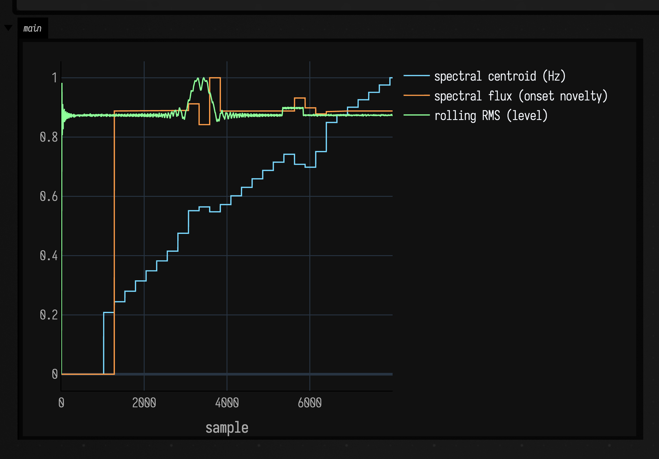
The smoothed centroid climbs with the chirp and the RMS tracks the overall level. The flux steps up as soon as its first window fills and then holds near the top of its range: each injected onset is a step of a percent or two above that plateau, not a spike, because all three traces are normalized to 0 … 1 for comparison and the flux never returns to its floor once the signal starts. SpectralCentroidFilter, SpectralRolloffFilter, SpectralFluxFilter, and RmsFilter all maintain their own ring buffer and recompute on each hop, so they behave like any other per-sample filter in the toolkit.

What else is in the family

• FFT — fft(...) / ifft(...) over DoubleArray, FloatArray, or List<Float>; forward and inverse; power-of-two (radix-2) or arbitrary length (Bluestein).
• Windows — WindowType.RECTANGULAR / HANN / HAMMING / BLACKMAN, via Windows.make(...).
• Spectrum — magnitude / power / phase / dB, binFrequency, peakFrequency, and the feature shortcuts centroid(), spread(), rolloff(), flatness().
• Spectrogram — stft(...), magnitudes(), centroidTrace() / rolloffTrace() / fluxTrace(), plus istft(...) for overlap-add reconstruction back to a signal.
• Features — SpectralFeatures.centroid / spread / rolloff / flux / flatness / rms / energy.
• Mel — Mel.hzToMel, Mel.melToHz, and a triangular Mel.filterBank(...) for perceptual / log-frequency band energies.
• Resonator bank (afield.audio.engine) — resonate(...) / ResonatorBank for a fixed complex filterbank at frequencies you choose, trackingResonate(...) / TrackingResonatorBank for resonators that lock onto and follow moving partials, with resonatorAlphaHeuristics(...) for per-frequency time constants.

Open the examples as a document

Every example on this page is also a starting point: open spectral_examples from the welcome screen and each box computes and draws its own figure with no other setup.

Then edit the signal, or swap WindowType.HANN for HAMMING / BLACKMAN, and re-run a box to watch its figure change.

The public declarations used on this page are listed, with their KDoc, in the codebase reference: timeseries.kt for the time-domain filters and detectors, spectral.kt for the frequency-domain half. Start from what's already in the box.