Looking at Data

How is the world divided up by time zone? We'll take the zones already on your machine and look at their UTC offsets: first as values, then as a distribution beside the code, then as a plot. Along the way you'll use .h, .h2 and Plotly. At the end we'll try a different kind of data: a value inside a GPU shader, changing too fast to print.

The time-zone examples run without a GPU. The final probe looks inside a compute shader; you can read it as a preview and come back to it after trying Graphics on the GPU.

Get some data

The data here is every time zone the JVM knows, with its offset from UTC on one day in January. It comes from java.time, so it is already on your machine. .h turns any value into a compact view, and .h2 opens the same value in an explorer you can scroll and expand:

:::static
import java.time.*

val day = Instant.parse("2026-01-15T12:00:00Z")
val zones = ZoneId.getAvailableZoneIds().sorted().associateWith {
    ZoneId.of(it).rules.getOffset(day).totalSeconds / 3600.0
}
val offsets = zones.values.toDoubleArray()

display("zones", zones.h)
display("browse", zones.h2)
display("offsets", offsets.h)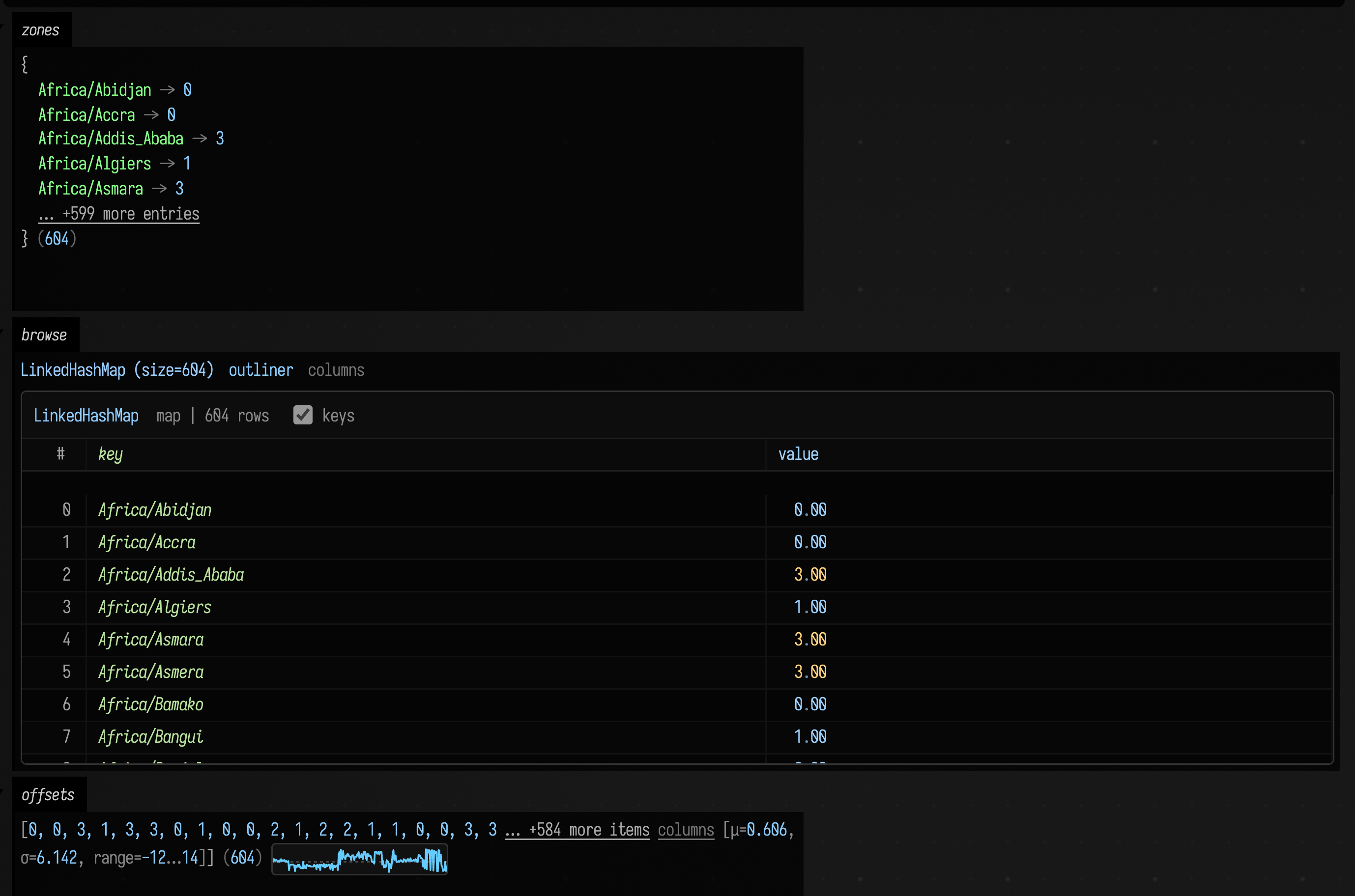

The compact view of offsets already says a lot: 604 zones, offsets from −12 to +14 hours, a mean a little east of Greenwich. .h2 pages its rows in as you scroll, so it costs the same for a map of six hundred entries or six million.

See the distribution

A mean and a spread do not say what shape the data has. To see the shape, draw it in the editor beside the code. __m("name") makes a marker: a named place on the line it is written on, which remembers the values you hand it. histogram(o, dur = ...) adds o to the marker and draws a histogram of what it holds just under that line; dur is how many of the most recent values it keeps, so dur = offsets.size keeps them all. stats does the same and adds the median, quartiles, skew and the values in the order they arrived:

:::static
import java.time.*

:::fold the zones and their offsets, as above
val day = Instant.parse("2026-01-15T12:00:00Z")
val zones = ZoneId.getAvailableZoneIds().sorted().associateWith {
    ZoneId.of(it).rules.getOffset(day).totalSeconds / 3600.0
}
val offsets = zones.values.toDoubleArray()

:::endfold

for (o in offsets) {
    __m("offsets").histogram(o, dur = offsets.size)
    __m("summary").stats(o, dur = offsets.size)
}

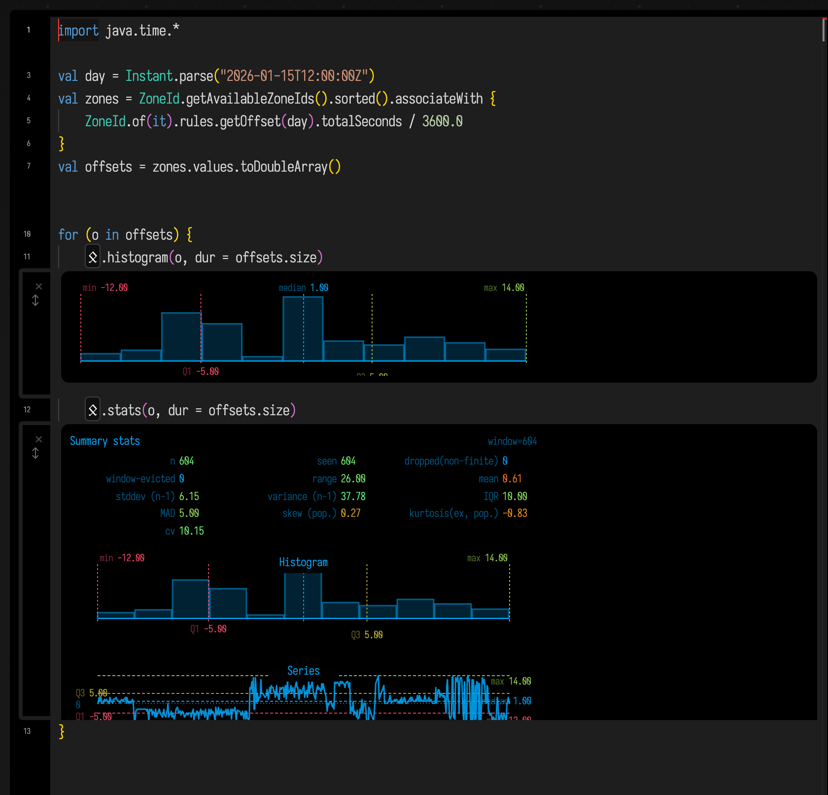
Two crowds: the Americas around five hours west of UTC, and Europe and Africa around one hour east, with Asia and the Pacific trailing out to +14. The same markers work inside a loop { }, where they keep a rolling window of the last dur values, which is how you watch a value that changes every frame.

Plot it

For a figure with axes, titles and hover, Field has Plotly. This counts the zones at each exact offset and draws the counts as bars, which shows what twelve bins could not: the zones that sit on a half or quarter hour.

:::static
import java.time.*
import space.kscience.plotly.*

:::fold the zones and their offsets, as above
val day = Instant.parse("2026-01-15T12:00:00Z")
val zones = ZoneId.getAvailableZoneIds().sorted().associateWith {
    ZoneId.of(it).rules.getOffset(day).totalSeconds / 3600.0
}
val offsets = zones.values.toDoubleArray()
:::endfold

val counts = offsets.toList().groupingBy { it }.eachCount().toSortedMap()

display(
    "plot",
    Plotly.plot {
            bar {
                x.set(counts.keys.toList())
                y.set(counts.values.toList())
            }
            layout {
                title = "time zones per UTC offset"
                xaxis { title = "hours from UTC" }
                yaxis { title = "zones" }
            }
        }
        .darkMode(),
)

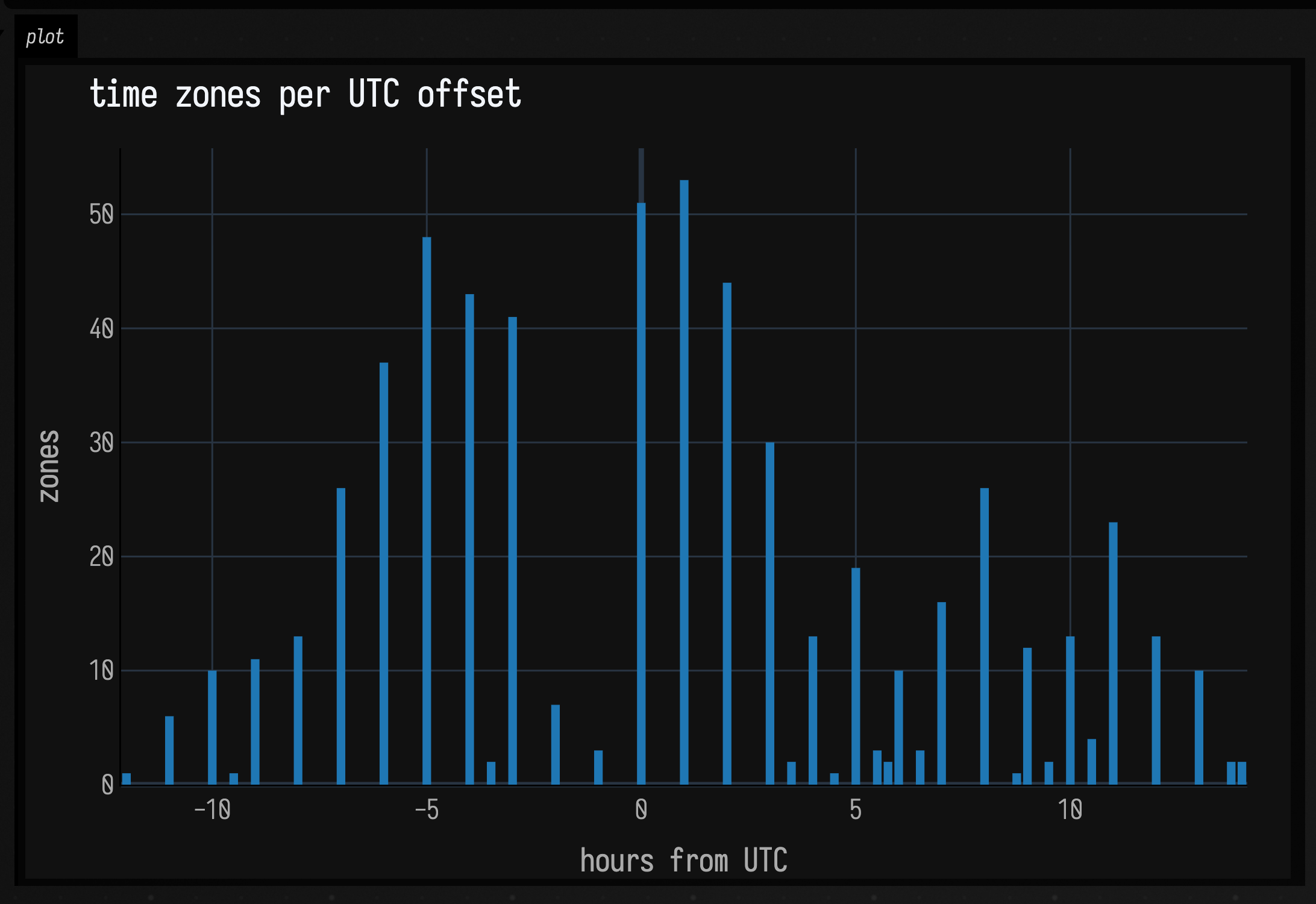
For a quick plot without the builder, linePlot(values) draws a list of numbers as a line and violin(values) draws their distribution; the visualization reference lists these and the rest. To draw a plot as geometry in the same drawing as your other lines, see Charts as FLines.

Probe a live value

How do you inspect a value inside a compute shader? Its particles live on the GPU, and a hundred thousand of them might change every frame. Add fieldProbe to the shader to record a value:

:::static
vec2 delta = moved - seed.xy; // moved: the particle's new position; seed: where it started
fieldProbe(length(delta));    // record how far it is from its start

Then turn the probe on from the box and show what it recorded:

:::static
fieldProbeHere(samples = 4096).display("probe")

The probe channel shows a panel that updates a few times a second while the particles move. It counts every value the shader recorded, says whether any were NaN or infinite, and draws a sample of them with the same summary panel as stats:

Field Probes has the whole particle system, and fieldStats, which computes the same statistics on the GPU and hands them back to the shader.

Where to go from here

• Visualizers & Controls has everything .h and .h2 draw (vectors, FLines, images, functions), the other inline markers, and the controls you can put beside a plot.
• Charts as FLines draws plots as geometry, with clickable marks and expect() for marking the range the data should stay in.
• DataFrames in a Box is for data that arrives as a table: Kotlin DataFrame with typed columns, shown with the same .h and .h2.
• The Drawing From Data section starts at Linear Algebra and goes on to functions, signals over time, simulation and spatial data.

Next on the Tour, Sound turns a pattern into something you can hear.