Spatial artificial life

Write a small local rule — count your neighbours, follow the strongest smell, grow toward the nearest unclaimed space — and a larger structure can appear: a spaceship, a coastline, a transport network, a dendrite with a fractional dimension. This page explores those systems through grids, continuous fields and populations of agents. For related work, see growing.kt, interaction nets, Wave Function Collapse, and graphs that change while you watch. For vehicles whose neurons have memory, adaptation and learning, see Braitenberg vehicles with memory.

Almost any local rule applied to noise looks organic, so each example here prints a measurement beside a control: the same setup with one ingredient removed, which gets the number wrong. A glider's every live cell is displaced by exactly (1, 1) after four generations, and the same seed under a rule one birth-count away is displaced by nothing at all. A flock of 400 agents reaches a polarization of 0.69 where 400 independent headings would give 0.044, and the same initial state with the alignment term zeroed reaches 0.073.

Source files

Six dependency-free files built on the existing imaging and mesh families. Nothing here reimplements convolution, connected-component labelling, colour mapping or marching cubes:

• alife.kt — IntGrid, the toroidal-or-bounded integer lattice; the grid↔Img bridges; and, mostly, the measurement layer that the rest of the family makes its claims through — polarization and its random baseline, blobShapes (the isoperimetric ratio that tells spots from stripes), correlationLength, topShare and massRadiusDimension.
• alife_ca.kt — LifeRule parsed from B3/S23, named Life patterns, exact cycle detection, cyclic multi-state CA, Wolfram's elementary 1-D rules as a space-time raster, and a 3-D life-like CA on IntVolume.
• alife_continuous.kt — mass-conserving diffusion, Gray–Scott reaction–diffusion, Gierer–Meinhardt Turing patterns, and Lenia.
• alife_agents.kt — boids, a Physarum deposit–sense–move population, and diffusion-limited aggregation with two control models.
• alife_lsystem.kt — a bracketed, parametric, optionally stochastic L-system with a turtle that emits FLines, and space-colonization branching.
• alife_field.kt — the inline ToHTML views, kept in their own file so the five above name nothing from Field's visualizer.

Two later files extend the agent side along an axis this page does not walk through. Every system above advances a whole population with one call and one parameter block, so two agents differ only in their state and never in what they are trying to do:

• alife_script.kt — ScriptWorld gives each agent its own suspending program on a fixed-step clock: forever, phase(name), parallel, moveUntil, and steering composed from whichever behaviours are active right now. The same seed gives the same run, bit for bit, across processes.
• alife_walls.kt — and an environment for it to run in: ScriptObstacle, swept circle collision with a per-agent WallResponse, avoidWalls and cling, and a radius-aware NavGrid so route() can go round a barrier that direct seek presses into. On an S-maze, over 96 agents, routed seek arrives 0.990 of the time against 0.000 for direct seek at the same budget.

Both are worked through in section 12, which also says where to find them as documents you can open and edit.

Limits:

• CPU only. These are reference implementations you can read. The GPU story is Field 4, StackSL and RectSL. Four systems from this family's neighbourhood do run on the GPU, as shaders you can edit: diffusion-limited aggregation, Biham–Middleton–Levine traffic, a lattice Boltzmann fluid and a forest fire.
• One named Lenia lifeform. Orbium ships with its published cells; the rest of Chan's catalogue loads from his animals.json if you supply it.
• O(N²) neighbour search in the agent models. A spatial hash is right for 50 000 agents and is a different piece of code; these flocks are a few hundred agents and legibility wins.
• Explicit Euler integration for the continuous systems, with the stability bound stated as a require rather than silently clamped.

1. Conway's Life

B3/S23 is the most-studied dynamical system in computing, which is exactly why it is the right place to start: there are facts about it to be checked. The glider translates one cell diagonally every four generations. The block is a still life. The blinker has period two. And the R-pentomino (five cells) runs for 1103 generations, peaks at a population of 319 at generation 821, and settles to 116 cells, six of which are gliders still flying away.

Those R-pentomino figures are about an unbounded board. On a board with walls the gliders are destroyed, and the system instead becomes exactly periodic at generation 1164 with 110 cells. Both answers are correct; they are answers to different questions. So the box below runs on a 620-wide board (wide enough that no glider can reach an edge in 1103 generations) and asserts liveBounds to confirm the walls never took part rather than assuming it.

:::static
// Conway's Life. Every claim here is about an object that predates this code, stated as an
// integer-grid equality rather than as an observation about a picture.
val glider = LifePatterns.glider.centeredOn(40, 40)
println("glider, 4 generations: rigid translation = " + translationBetween(glider, glider.stepTimes(LIFE, 4)))
println("glider, 8 generations: rigid translation = " + translationBetween(glider, glider.stepTimes(LIFE, 8)))

// The control: one birth count away and the same seed is not a spaceship at all.
println(
    "same seed under B34/S23, 4 generations: " + translationBetween(glider, glider.stepTimes(lifeRule("B34/S23"), 4)),
)

val block = LifePatterns.block.centeredOn(20, 20)
println("block is bit-identical after one step: " + block.step(LIFE).sameCellsAs(block))
println("blinker's detected period: " + LifePatterns.blinker.centeredOn(20, 20).runUntilCycle(LIFE, 20).period)
println("toad's detected period: " + LifePatterns.toad.centeredOn(20, 20).runUntilCycle(LIFE, 20).period)

/*
The R-pentomino. The textbook figures -- peak 319 at generation 821, then 116 cells from
generation 1103 -- are facts about an UNBOUNDED board: six of those 116 cells are gliders still
in flight. So it needs room. 620 wide gives every glider more than the 1103/4 cells it can
travel, and liveBounds() confirms nothing reached an edge rather than assuming it.
*/
var g = LifePatterns.rPentomino.centeredOn(620, 620, wrap = false)
var peak = 0
var peakAt = 0
for (gen in 1..1103) {
    g = g.step(LIFE)
    val pop = g.population()
    if (pop > peak) {
        peak = pop
        peakAt = gen
    }
}
val b = g.liveBounds()!!
println("R-pentomino peak population " + peak + " at generation " + peakAt)
println(
    "population at generation 1103 = " + g.population() + ", live cells " + b[0] + " clear of the board edge",
)

:::fold draw the glider's first five generations, twelve pixels to a cell
showImg(
    montage(
        (0..4).map {
            "gen " + it to LifePatterns.glider.centeredOn(16, 16).stepTimes(LIFE, it).toImg(2).upscaleNearest(12)
        },
        columns = 5,
        cellSide = 200,
    ),
    caption = "one glider, five generations: the same shape displaced by (1, 1)",
)
:::endfold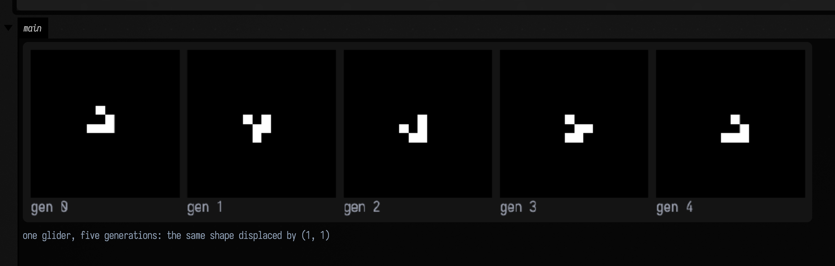

translationBetween is not a centroid comparison. It aligns the two patterns' bounding boxes, shifts one by that offset, and then demands exact cell-by-cell equality, so a pattern that moved and changed shape returns null. A wrong rule cannot fluke that: the B34/S23 line above prints null.

The two objects, moving

Two panels, 400 generations, two generations per displayed frame: slow enough that the glider's four-generation cycle is legible rather than a strobe.

Left: the glider, on a 16-cell torus, twenty-four pixels to a cell. It laps that board every 64 generations and does it six times over, so if you watch one edge you see it leave and re-enter from the other. That is the same claim the montage above makes, and the same claim translationBetween asserts, in the form where it is obvious.

Right: the R-pentomino on a 64-cell walled board, with its live population in the caption. This is the walled question, not the unbounded one the numbers above are about: those need 620 cells, and 620 cells at one pixel each is a video whose interesting part is four pixels wide. Same rule, same seed, different board, and what it shows is the shape of the thing: five cells, a violent expansion, then a long quieting-down toward something stationary.

:::static
:::fold the two boards, integer-upscaled so a cell is a block you can count
/*
Both boards are integer-upscaled to the same 384 pixels, so a cell is a block you can count:
twenty-four pixels for the glider's 16-cell torus, six for the R-pentomino's 64-cell walled
board.
*/
fun boards(g: IntGrid, r: IntGrid, n: Int) = [
    "glider, gen " + n to g.toImg(2).upscaleNearest(24),
    "R-pent " + n + ": " + r.population() + " live" to r.toImg(2).upscaleNearest(6),
]

:::endfold

/*
400 generations over 200 displayed frames: TWO generations per frame. Slower than every other
clip on this page -- the glider's period is FOUR generations, and a spaceship stepped
nine generations at a time is a strobe rather than a spaceship.
*/
animateEvolution(
    LifePatterns.glider.centeredOn(16, 16) to LifePatterns.rPentomino.centeredOn(64, 64, wrap = false),
    totalSteps = 400,
    seconds = 7.0,
    framesTarget = 200,
    columns = 2,
    cellSide = 384,
    step = { (g, r) -> g.step(LIFE) to r.step(LIFE) },
    panels = { (g, r), n -> boards(g, r, n) },
)

2. Wolfram's elementary rules

A one-dimensional automaton's behaviour is two-dimensional, so elementaryCa returns the whole space-time diagram as an IntGrid: one row per generation, time downward. Every famous statement about these 256 rules is a statement about this picture.

Rule 90 is left XOR right, and from a single seed its space-time diagram is Pascal's triangle mod 2, the Sierpiński gasket. sierpinskiReference computes that from Kummer's theorem (C(n, k) is odd exactly when n and k == k) without running a cellular automaton at all. So the equality between them is a cross-check between two unrelated computations, not a stepper agreeing with itself, and it holds in all 32 896 cells. A second, independent oracle comes free: row g of that diagram holds exactly 2^popcount(g) live cells (Gould's sequence).

Rule 184 is the traffic rule, and it conserves the number of live cells exactly, forever. Rule 90 does not, which is the control that stops "184 conserves density" from being a property of the harness.

:::static
/*
Wolfram's elementary rules, and the sharpest evidence in the family: rule 90 from a single seed
IS Pascal's triangle mod 2, and `sierpinskiReference` computes that from Kummer's theorem
without running a cellular automaton at all. The equality is a cross-check between two
unrelated computations rather than a stepper agreeing with itself.
*/
val w = 257
val gens = 128
val rule90 = elementaryCa(90, w, gens)
val oracle = sierpinskiReference(w, gens)
var differing = 0
for (i in rule90.cells.indices) if (rule90.cells[i] != oracle.cells[i]) differing++
println("rule 90 vs Pascal mod 2: " + differing + " differing cells of " + rule90.cells.size)

// A second, independent oracle: row g of that diagram holds exactly 2^(popcount g) live cells.
val rows = (0 until gens).map { r -> (0 until w).count { rule90.cells[r * w + it] == 1 } }
println(
    "row populations are exactly 2^popcount(generation): " +
        (rows == (0 until gens).map { 1 shl Integer.bitCount(it) }),
)

// Rule 184 is the traffic rule: it conserves the number of 1s exactly, forever.
val seedRow = IntArray(257) { if ((it * 7919) % 3 == 0) 1 else 0 }
val traffic = elementaryCa(184, 257, 200, seedRow)
val pops = (0 until 200).map { r -> (0 until 257).count { traffic.cells[r * 257 + it] == 1 } }
println("rule 184 distinct row populations over 200 generations: " + pops.distinct())
println("rule 90 distinct row populations: " + rows.distinct().size + " values, so NOT conserved")

val col30 = elementaryCa(30, 601, 600).centerColumn()
println(
    "rule 30 centre column: " +
        col30.count { it == 1 } +
        "/600 ones, longest run " +
        longestRunLength(col30) +
        " (rule 90's is " +
        longestRunLength(rule90.centerColumn()) +
        ")",
)

:::fold draw four of the 256 space-time diagrams, time downward
showImg(
    montage(
        [
            "rule 90 = Pascal mod 2" to rule90.toImg(2),
            "rule 30" to elementaryCa(30, 257, 128).toImg(2),
            "rule 110 (universal)" to
                elementaryCa(110, 257, 128, IntArray(257) { if (it % 13 == 0) 1 else 0 }).toImg(2),
            "rule 184 (density-conserving)" to traffic.toImg(2),
        ],
        columns = 2,
        cellSide = 300,
    ),
)
:::endfold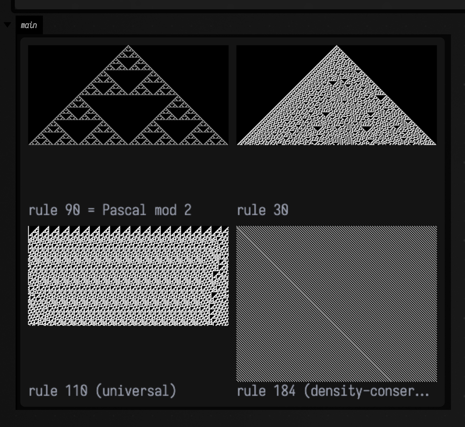

Four rules, drawn a generation at a time

A space-time diagram is a picture of time, which makes animating one slightly strange: the motion is the downward growth of the picture, not motion within it. It pays off anyway, because the four panels grow at the same rate and the differences between the 256 rules become differences you can watch appear.

One generation per displayed frame, 128 generations in six seconds. Rule 90 lays down the Sierpiński gasket with the self-similarity arriving in bursts at the powers of two: the row populations are 2^popcount(g), so the widest rows are the ones where g has many bits, and the diagram visibly breathes. Rule 30 starts identically, from a single cell, and never repeats. Rule 110, the universal one, separates into a background of periodic structure with localised gliders travelling through it, which is what a proof of universality has to be built out of. Rule 184 just shifts, forever, conserving its 86 live cells exactly.

:::static
:::fold compute the four space-time diagrams once, in full
// Compute the four space-time diagrams once, in full: 257 cells wide, 128 generations tall.
val seedRow = IntArray(257) { if ((it * 7919) % 3 == 0) 1 else 0 }
val diagrams = [
    "rule 90" to elementaryCa(90, 257, 128).toImg(2),
    "rule 30" to elementaryCa(30, 257, 128).toImg(2),
    "rule 110" to elementaryCa(110, 257, 128, IntArray(257) { if (it % 13 == 0) 1 else 0 }).toImg(2),
    "rule 184" to elementaryCa(184, 257, 128, seedRow).toImg(2),
]

:::endfold

/*
128 generations over 128 displayed frames: ONE row of every diagram per frame. The upscale comes
AFTER the reveal, so `n` counts generations rather than pixels -- and `rowsRevealed` keeps the
full height, so montage frames each panel identically instead of rescaling a growing image.
*/
animateEvolution(
    Unit,
    totalSteps = 128,
    seconds = 6.0,
    framesTarget = 128,
    columns = 2,
    cellSide = 520,
    step = { it },
    panels = { _, n ->
        diagrams.map { (name, img) -> name + ", gen " + n to img.rowsRevealed(n).upscaleNearest(2) }
    },
)

3. Cyclic cellular automata

A cyclic cellular automaton has k states arranged in a ring. A cell in state s advances to s + 1 as soon as at least threshold of its neighbours are already in s + 1; otherwise it waits. Nothing can skip a state, and there is no way back, so the only durable structures are rotating bands.

The measurement that makes "it self-organised" checkable is cyclicAdvanceFraction. In an uncorrelated soup a cell can advance exactly when one of its eight Moore neighbours happens to hold its successor state, which is 1 - (1 - 1/k)^8: a closed form, not a threshold. For k = 14 that is 0.4473, and the measurement is 0.4483. Four hundred generations later every cell is being driven by a neighbour and the fraction pins at 1.0000, which is something no uncorrelated field does at any k.

The second pair of panels is the excitable corner of the parameter space (six states, threshold three, radius two), which curls into visible spiral cores. That is a different phase, and the difference is reported as a length scale rather than left to the eye, though note the direction: the wider neighbourhood gives the smaller correlation length, because the spiral arms are narrow.

:::static
/*
A cyclic cellular automaton: a cell in state s advances to s+1 as soon as any neighbour is
already in s+1. Nothing can skip, so the only durable structures are rotating bands.

The measurement that makes "it self-organised" checkable: in an UNCORRELATED soup a cell can
advance exactly when one of its 8 Moore neighbours happens to hold its successor state, which
is 1 - (1 - 1/states)^8 -- a closed form. Once the field has organised, every cell is driven by
a neighbour and the advance fraction pins at 1.0, which no uncorrelated field does.
*/
val rule = CYCLIC_LABYRINTH
val soup = IntGrid.random(200, 200, states = rule.states, seed = 7L)
val predicted = 1.0 - Math.pow(1.0 - 1.0 / rule.states, 8.0)
val early = cyclicAdvanceFraction(soup, soup.step(rule))
val settled = soup.stepTimes(rule, 400)
val late = cyclicAdvanceFraction(settled, settled.step(rule))
println("soup advance fraction " + early.f4 + ", closed form " + predicted.f4)
println("after 400 generations " + late.f4 + " of cells advance every step")

// The excitable corner of the parameter space (wider neighbourhood, higher threshold) is a
// visibly different phase -- spiral cores -- and the difference is measurable as a length scale.
val ex = CYCLIC_EXCITABLE
val exSettled = IntGrid.random(200, 200, states = ex.states, seed = 7L).stepTimes(ex, 200)
println(
    "correlation length: labyrinth " +
        settled.toImg(rule.states).correlationLength(maxLag = 30).f2 +
        ", excitable " +
        exSettled.toImg(ex.states).correlationLength(maxLag = 30).f2,
)

:::fold one palette per rule, and three generations of the labyrinth beside the excitable phase
val palette = cyclicPalette(rule.states)
showImg(
    montage(
        [
            "gen 0 (soup)" to soup.toImg(palette),
            "gen 40" to soup.stepTimes(rule, 40).toImg(palette),
            "gen 400" to settled.toImg(palette),
            "excitable, gen 200" to exSettled.toImg(cyclicPalette(ex.states)),
        ],
        columns = 2,
        cellSide = 280,
    ),
)
:::endfold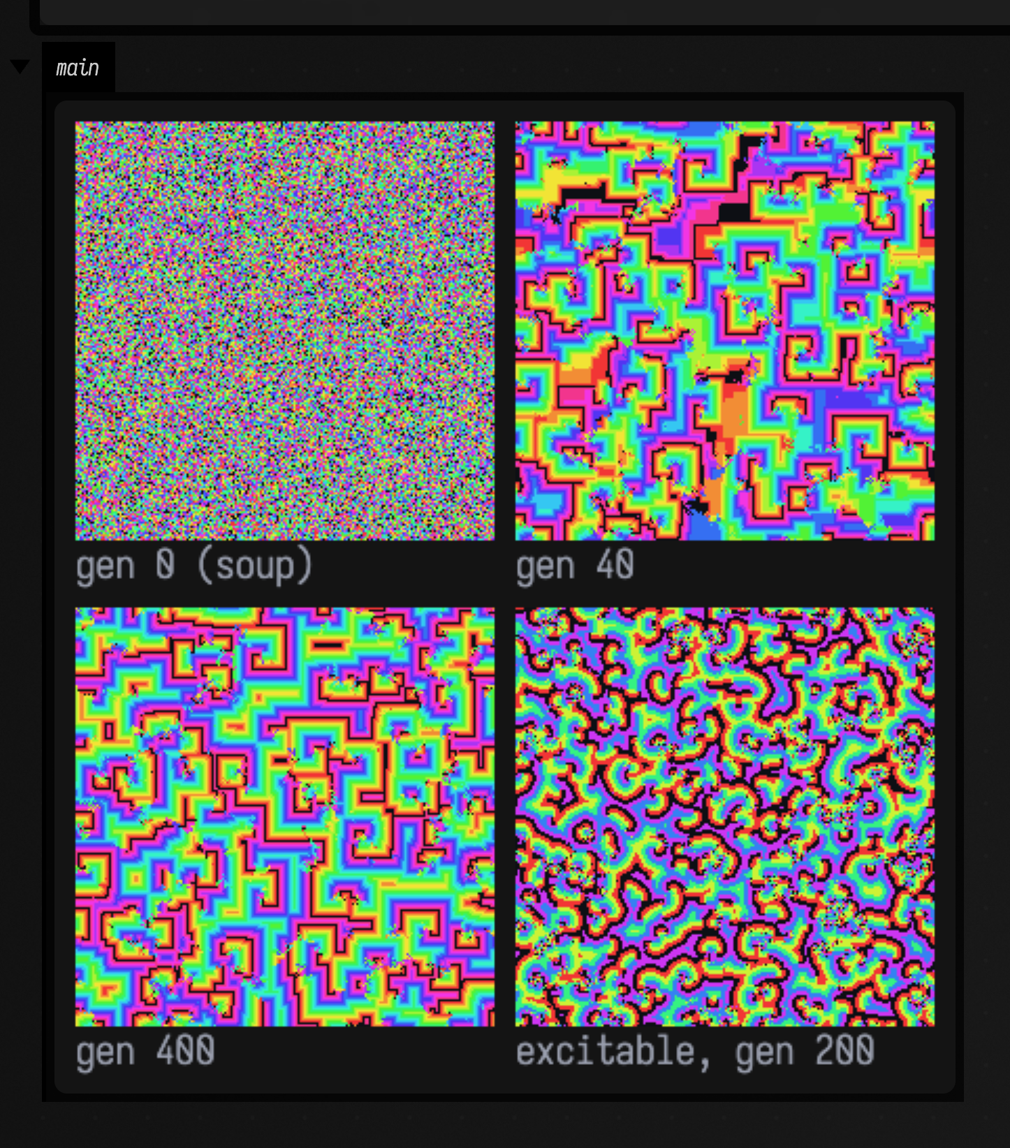

The two phases, running

Of everything in this family the cyclic CA is the system whose stills lie hardest, because the whole point of it is rotation and a still frame has no chirality. Both panels below run 400 generations in six and a half seconds (a little over three generations per displayed frame) from the same kind of soup. The lattices are 96 cells rather than the figure's 200, drawn three pixels to a cell: at one pixel per cell a rotating spiral core is about four pixels of video and reads as flicker.

The left panel is the sequence the figure above samples at generations 0, 40 and 400, without the gaps. Watch for the transition, because it is sharp and it has a name: the soup is locally advancing everywhere (that is the 0.4483 the box prints, and it is what an uncorrelated field gives) but it has no structure, and then within a few dozen generations it is entirely bands, after which every cell advances on every step forever. Nothing directs that. The right panel is the excitable rule, and what it does that the labyrinth does not is rotate: those spiral cores are pinned defects, they wind at a fixed rate, and you cannot see any of that in a photograph of one.

:::static
:::fold one palette per rule, fixed by the rule and never by the frame
/*
One palette per rule, FIXED -- it is a function of the rule's state count, never of the frame,
which is what makes generation 0 and generation 400 the same picture of the same thing. Three
pixels to a cell, nearest-neighbour, so the bands are countable and the encoder sees flat blocks.
*/
val pal = cyclicPalette(CYCLIC_LABYRINTH.states)
val exPal = cyclicPalette(CYCLIC_EXCITABLE.states)
fun soups(a: IntGrid, b: IntGrid, n: Int) = [
    "labyrinth, gen " + n to a.toImg(pal).upscaleNearest(3),
    "excitable, gen " + n to b.toImg(exPal).upscaleNearest(3),
]

:::endfold

// Two cyclic rules from the same kind of soup, stepped together so the schedule is shared:
// 400 generations over 130 displayed frames, so a little over THREE generations per frame.
val rule = CYCLIC_LABYRINTH
val ex = CYCLIC_EXCITABLE
animateEvolution(
    IntGrid.random(96, 96, states = rule.states, seed = 7L) to IntGrid.random(96, 96, states = ex.states, seed = 7L),
    totalSteps = 400,
    seconds = 6.5,
    framesTarget = 130,
    columns = 2,
    cellSide = 288,
    step = { (a, b) -> a.step(rule) to b.step(ex) },
    panels = { (a, b), n -> soups(a, b, n) },
)

4. Gray–Scott reaction–diffusion

Two coupled fields, u (substrate) and v (autocatalyst), the reaction U + 2V → 3V with V → P, and two numbers: a feed rate F and a kill rate k. The entire zoo of morphologies is a function of those two numbers. Two knobs producing that much variety is why Gray–Scott is the canonical morphogenesis model.

Spots and a labyrinth can have identical coverage, identical mean and identical variance. Nothing in a histogram separates them. What does separate them is the shape of their features, and morphology() measures it: the isoperimetric ratio \( P^2/4\pi A \) (1 for a disc, growing without bound as a region gets thinner and more convoluted) and the share of the covered area held by the single largest connected feature.

The numbers below, from the run in the box: the spots preset gives 329 separate features with a median ratio of 0.80 and a largest-blob share of 0.008; the two labyrinth presets give 24 and 34 features with ratios of 2.5 and 2.4 and largest shares of 0.64 and 0.45. Three times less round, and dominated by one connected structure. The holes preset is the inverse morphology and reads as a single blob at 0.78 coverage with a ratio of 90.

Two controls. v = 0 is a stable fixed point of the equations, so an unseeded field stays at exactly 0.0 forever, so the pattern comes from the dynamics and not from the renderer. And with Du == Dv the Turing instability's short-scale advantage is gone and the same seed, the same reaction and the same 6000 steps produce nothing at all: Turing's own argument, restated as an experiment.

:::static
/*
Gray-Scott reaction-diffusion. Two coupled fields, two parameters, and the whole zoo of
morphologies -- spots, worms, mazes, holes -- is a function of those two numbers.

The point of `morphology()` is that a regime claim should be a claim about numbers. Spots and a
labyrinth can have identical coverage, identical mean and identical variance; what separates
them is the SHAPE of their features (isoperimetric ratio P^2/4piA, ~1 for a disc) and whether
one connected structure dominates.
*/
val side = 128
val steps = 6000
val runs =
    [
            "spots 0.030/0.062" to GRAY_SCOTT_SPOTS,
            "worms 0.037/0.060" to GRAY_SCOTT_WORMS,
            "maze 0.029/0.057" to GRAY_SCOTT_MAZE,
            "holes 0.039/0.058" to GRAY_SCOTT_HOLES,
        ]
        .map { (label, p) ->
            label to grayScottSeed(side, side, patches = 6, patchSize = 14, seed = 11L).stepTimes(p, steps)
        }
for ((label, end) in runs) println(label + " -> " + end.v.morphology())

/*
Two controls. v = 0 is a fixed point of the equations, so an unseeded field never patterns;
and equal diffusion coefficients destroy the Turing instability entirely, which is Turing's
own argument restated as an experiment.
*/
val unseeded = grayScottSeed(side, side, patches = 0).stepTimes(GRAY_SCOTT_WORMS, 500)
println("CONTROL no seed: max autocatalyst after 500 steps = " + unseeded.v.max())
val equalD =
    grayScottSeed(side, side, patches = 6, patchSize = 14, seed = 11L)
        .stepTimes(GrayScottParams(feed = 0.037, kill = 0.060, du = 0.08, dv = 0.08), steps)
println("CONTROL Du == Dv -> " + equalD.v.morphology())

:::fold draw the four regimes and the two controls, all on one fixed magma range
val controls: List<Pair<String, GrayScottState>> = [
    "CONTROL no seed" to unseeded,
    "CONTROL Du == Dv" to equalD,
]
showImg(
    montage(
        (runs + controls).map { (label, s) ->
            label to s.v.colormap("magma", 0f, 0.5f).upscaleNearest(2)
        },
        columns = 3,
        cellSide = 260,
    ),
)
:::endfold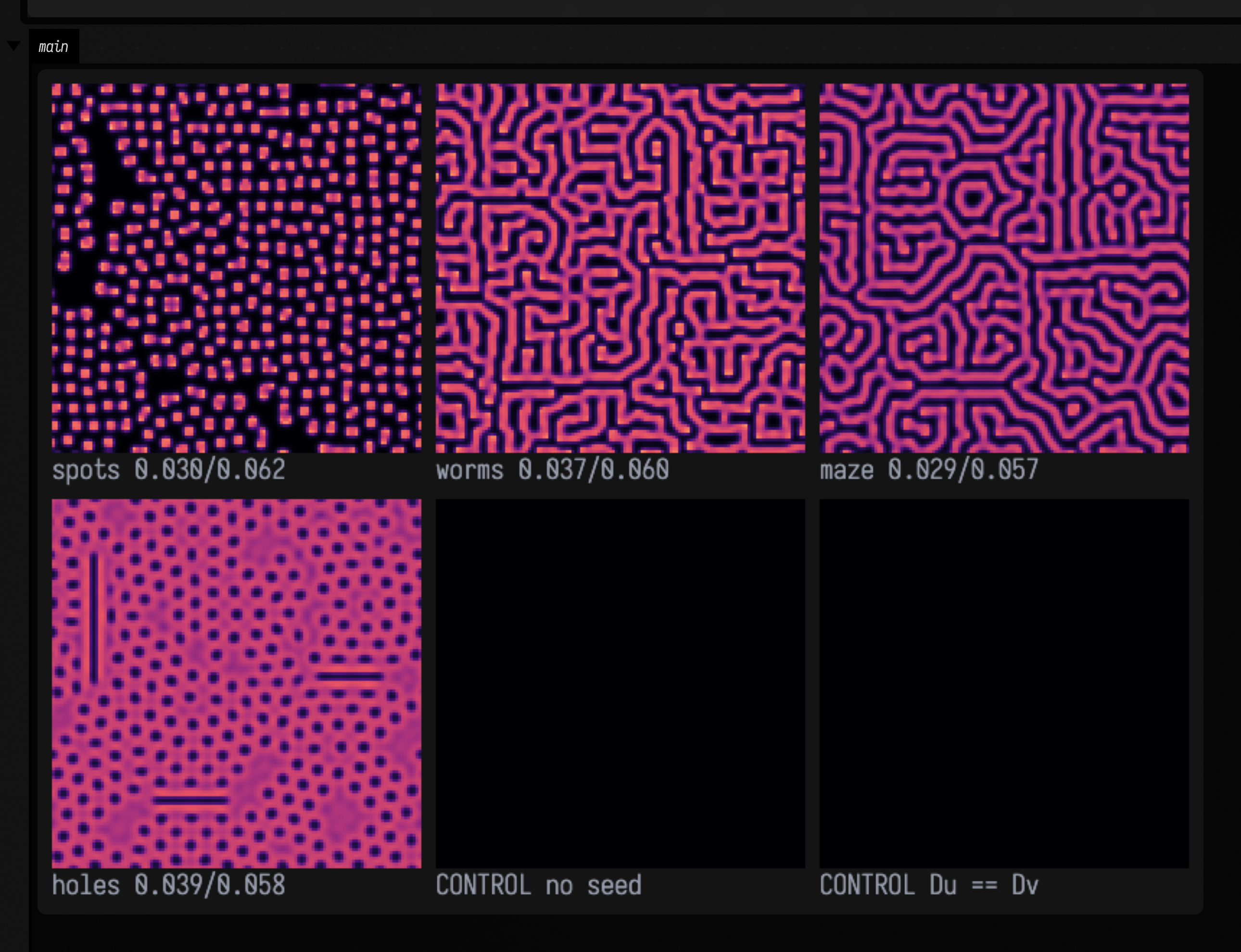

The same 6000 steps, recorded live

A montage of finished fields is the evidence, and it is also the one view that hides what reaction–diffusion is: those numbers are the end of a process, and the process is the phenomenon. So here is one preset again, animated: the maze field, F = 0.029, k = 0.057, the same 6000 steps.

What to watch, with the step counter in the caption as your clock:

• Step 63. Six square seed patches, each with a bright rim. That is grayScottSeed's output plus enough steps to make it visible: v is high only where the patch meets the substrate.
• Step ~600. Every square has buckled into a four-lobed cross. This is the Turing instability arriving as an event: the flat patch boundary is unstable, and it does not decay into noise, it picks a wavelength. The four lobes are that wavelength meeting the square's symmetry.
• Step ~1600. Each patch has filled its own interior with labyrinth and the fronts are advancing into empty substrate. The black regions are unconsumed u, and they are shrinking.
• Step ~2900. The fronts have met. From here the field is entirely labyrinth and the dynamics change character completely: no more growth, only rearrangement.
• Step 6000. Annealed. Watch the last second and almost nothing moves; the little that does is at the free ends, which is where a labyrinth still has somewhere to go. That is why the section's numbers are stable enough to assert.

Those five events are not spread evenly through the 6000 steps, so the clip is not paced evenly either.

:::static
:::fold the autocatalyst field, on a fixed colour range
/*
The autocatalyst field on a FIXED 0..0.5 magma range. Auto-ranging per frame is what makes an
animation of a growing pattern appear to stand still, and it is the single easiest way to turn
a reaction-diffusion clip into a lie.
*/
fun view(s: GrayScottState, n: Int) =
    ["maze - step " + n + " of 6000" to s.v.colormap("magma", 0f, 0.5f).upscaleNearest(3)]

:::endfold

/*
The `maze` preset, the same 6000 steps the figure above measures, over 140 displayed frames --
but NOT 43 steps per frame. `ramp = 40` makes the last displayed frame advance forty times as
many steps as the first, which is the schedule a log-time process needs: the mid-point of the
clip is step 819 rather than step 3000. This is the number to change if you disagree.
*/
animateEvolution(
    grayScottSeed(128, 128, patches = 6, patchSize = 14, seed = 11L),
    totalSteps = 6000,
    seconds = 7.0,
    ramp = 40.0,
    cellSide = 420,
    step = { it.step(GRAY_SCOTT_MAZE) },
    panels = { s, n -> view(s, n) },
)

5. Lenia

Lenia is a cellular automaton whose cells hold any value from 0 to 1 instead of on or off. Each step, every cell takes a weighted average of its neighbourhood out to radius R (the kernel K), passes it through a growth curve G that is positive near one value mu and negative elsewhere, and moves a small step dt in that direction:

A  <-  clamp(A + dt * G(K * A), 0, 1)

What makes Lenia worth studying is that some patterns under some rules behave like creatures: they keep their shape and move. The best known is Orbium unicaudatus, from Bert Chan's catalogue of Lenia lifeforms. LeniaPresets.orbium() loads its rule and its 20 × 20 array of cells from that catalogue. On the left below it glides across a 64-cell torus at a steady 0.62 cells per step, and its mass (the field's mean value, in the caption) stays level the whole way. On the right are the same cells under the same rule with one number changed: mu, the centre of the growth curve, moved from 0.15 to 0.12. The creature swells into a ring, the ring tears, and the pieces multiply until they cover the torus.

:::static
val orbium = LeniaPresets.orbium()

:::fold draw both fields on a fixed 0..1 inferno scale, with the mean field in the caption
fun fields(a: Img, b: Img, n: Int) = [
    "Orbium, step %d: mass %.4f".format(n, a.mean()) to a.colormap("inferno", 0f, 1f).upscaleNearest(6),
    "mu 0.12, step %d: mass %.4f".format(n, b.mean()) to b.colormap("inferno", 0f, 1f).upscaleNearest(6),
]

:::endfold

// The same cells, with the growth curve centred at 0.12 instead of 0.15.
val lowMu = leniaRuleFromCatalogue(radius = 13, t = 10.0, mu = 0.12, sigma = 0.015)

// At Orbium's 0.62 cells per step, 200 steps is about two laps of the 64-cell torus.
animateEvolution(
    orbium.seed(64, 64) to orbium.seed(64, 64),
    totalSteps = 200,
    seconds = 7.0,
    columns = 2,
    cellSide = 384,
    step = { (a, b) -> a.leniaStep(orbium.rule) to b.leniaStep(lowMu) },
    panels = { (a, b), n -> fields(a, b, n) },
)

Orbium's rule is R = 13, dt = 1/10, mu = 0.15, sigma = 0.015, with the polynomial kernel and growth curve its catalogue entry names. leniaRuleFromCatalogue builds any rule in that catalogue's terms, and leniaCreatures reads a whole catalogue file, so the other creatures in Chan's animals.json load the same way.

Moving the growth window

The shape is the creature: shuffle Orbium's 400 values into a random arrangement, keeping its mass and its histogram, and under the same rule the patch dies, in every one of the six shuffles the box below tries. And the creature lives in a band of rules, not at one point. Run the same cells with only mu changed: from 0.13 to 0.16 Orbium survives and glides. At 0.12 the growth curve rewards thinner neighbourhoods, and it bursts into a field of about 25 fragments that covers the torus. At 0.17 and above it needs a denser neighbourhood than it has, and it shrinks and dies. The rows below are 0.12, 0.15 and 0.18, each at steps 0, 5, 10, 20 and 250.

:::static
val orbium = LeniaPresets.orbium()
for (seed in 1L..6L) {
    println(
        "shuffled cells, seed " + seed + ": " + leniaRun(orbium.shuffled(seed).seed(64, 64), orbium.rule, steps = 300),
    )
}
for (mu in [0.11, 0.12, 0.13, 0.16, 0.17, 0.18]) {
    val rule = leniaRuleFromCatalogue(radius = 13, t = 10.0, mu = mu, sigma = 0.015)
    println("mu = " + mu + ": " + leniaRun(orbium.seed(64, 64), rule, steps = 300))
}

:::fold three values of mu, the same five moments of each
val moments = [0, 5, 10, 20, 250]
val panels =
    [0.12, 0.15, 0.18].flatMap { mu ->
        val rule = leniaRuleFromCatalogue(radius = 13, t = 10.0, mu = mu, sigma = 0.015)
        var current = orbium.seed(64, 64)
        var done = 0
        moments.map { step ->
            current = current.leniaTimes(rule, step - done)
            done = step
            (if (step == 0) "mu " + mu else "step " + step) to current.colormap("inferno", 0f, 1f).upscaleNearest(3)
        }
    }
showImg(
    montage(panels, columns = 5, cellSide = 192),
    caption = "rows: mu = 0.12, 0.15, 0.18; columns: steps 0, 5, 10, 20 and 250",
)
:::endfold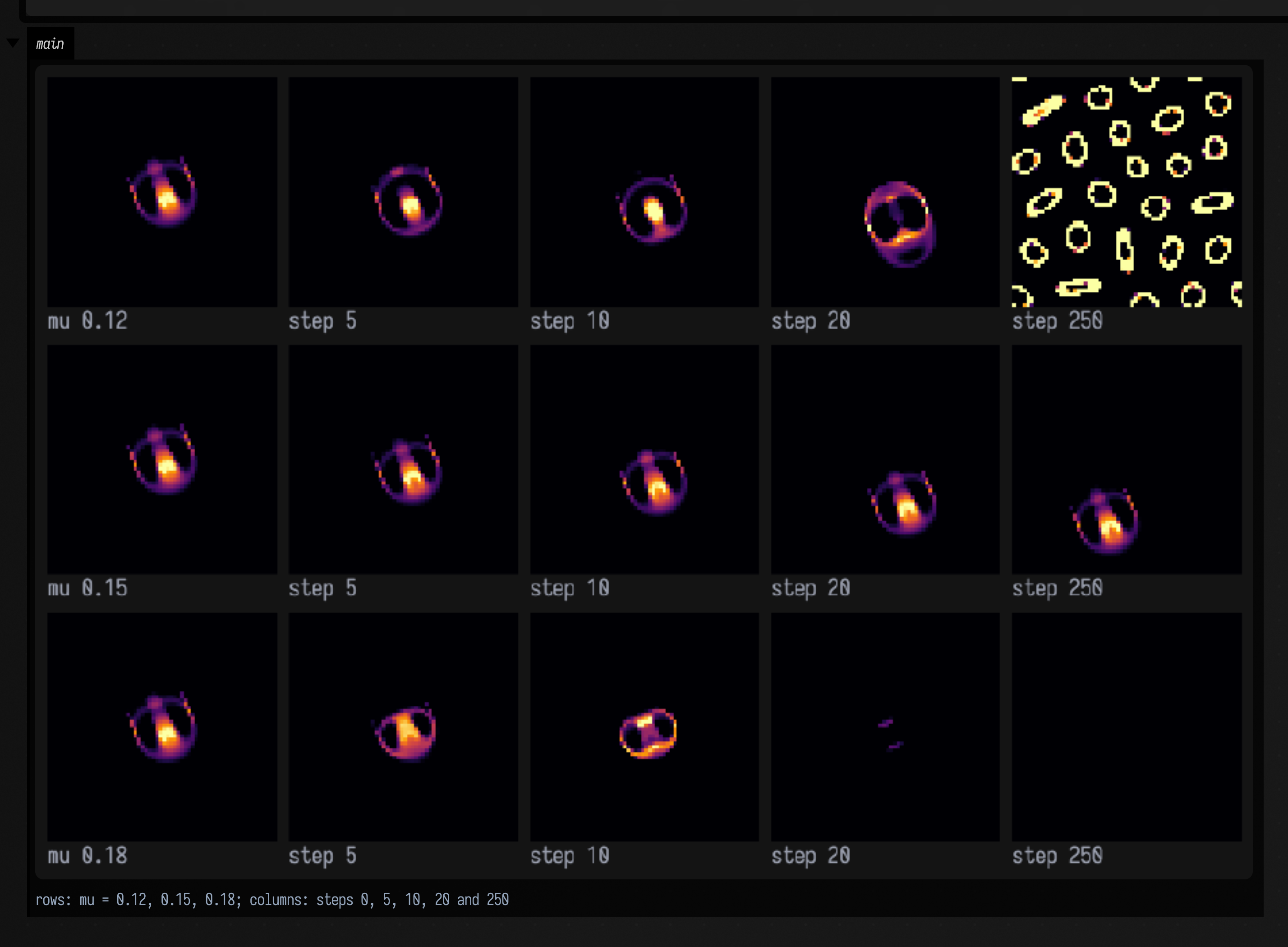

Checking the implementation against Life

Lenia has a limit in which it becomes an ordinary on/off automaton, and that gives a check on the code. With a kernel that weights the eight neighbours equally, dt = 1, and a growth curve that is +1 on the birth counts, 0 on survive-only counts and -1 elsewhere, every step lands each cell exactly on 0 or 1 and Lenia is an outer-totalistic B/S rule. So this file's float convolution and alife_ca.kt's integer neighbour counting must agree bit for bit. leniaFromLifeRule builds that limit, and over 20 generations of a glider the largest per-cell difference is 0.0. Moving the growth window by one neighbour count makes them disagree completely.

This checks the two update mechanisms against each other, not the rule: leniaFromLifeRule reads the same B3/S23 tables the integer stepper reads, so a wrong table would give two wrong steppers in perfect agreement. The rule is checked separately, in section 1, against facts about Life from the literature: the glider moves (1, 1) every four generations, the block stays still, the blinker has period 2. The limit also needs birth ⊆ survive, because a count that births a dead cell but kills a live one cannot be written as a growth curve of the count alone, so leniaFromLifeRule rejects such a rule rather than building a different automaton.

:::static
val discrete = leniaFromLifeRule(LIFE)
println("discrete-limit kernel: " + discrete.taps.size + " taps summing to " + discrete.taps.weight.sum())

var grid = LifePatterns.glider.centeredOn(32, 32)
var field = grid.toImg(2)
var worst = 0.0
for (gen in 1..20) {
    grid = grid.step(LIFE)
    field = field.leniaTimes(discrete, 1)
    worst = maxOf(worst, fieldMaxAbsDiff(field, grid.toImg(2)))
}
println("20 generations, float Lenia vs integer Life: worst per-cell difference " + worst)
println(
    "the glider the float stepper carried moved by " +
        translationBetween(LifePatterns.glider.centeredOn(32, 32), field.toIntGrid(0.5f)),
)

// Control: move the growth window by one neighbour count and nothing else.
println(
    "CONTROL, growth window at B4/S234: difference " +
        fieldMaxAbsDiff(
            LifePatterns.glider.centeredOn(32, 32).toImg(2).leniaTimes(leniaFromLifeRule(lifeRule("B4/S234")), 20),
            grid.toImg(2),
        ),
)

:::fold draw both steppers' glider after 20 generations
showImg(
    montage(
        [
            "float Lenia, gen 20" to field.upscaleNearest(8),
            "integer Life, gen 20" to grid.toImg(2).upscaleNearest(8),
        ],
        columns = 2,
        cellSide = 256,
    ),
)
:::endfold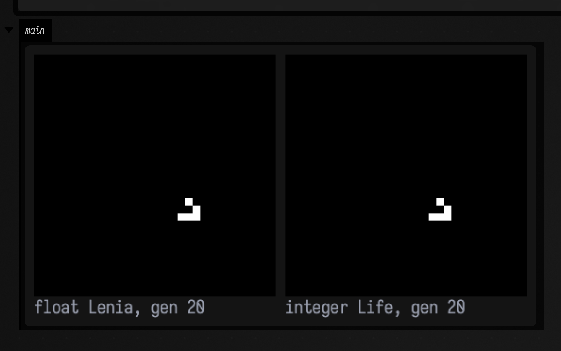

6. Boids

Reynolds' three rules — separation, alignment, cohesion — on a torus. The domain wraps for a reason beyond tidiness: in a bounded box the walls do half the flocking, because agents that bounce off the same wall end up parallel, so a polarization measured in a box is not evidence about the rules.

A flock is two things at once, and both are measured here:

• Aligned. The order parameter \( \lvert \sum \hat{v} \rvert / N \) is 0.692 after 900 steps. That needs a scale, so randomPolarizationBaseline gives it: \( \sqrt{\pi} / 2\sqrt{N} \) is the expected value for N independent headings, which for 400 agents is 0.044. The measured value is 15.6× that. And the same initial state with alignmentWeight = 0, nothing else changed, reaches 0.073.
• Spaced. The 5th-percentile nearest-neighbour distance is 1.37 cells; with separationWeight = 0 it collapses to 0.01. The floor under that distribution is the separation term, and you can see the control arm's population has collapsed to points.

0.692 rather than something near 1 is the correct answer, not a weak one: the population settles into several separate flocks with different headings (visible in the figure), and the global order parameter of k independent flocks tops out near \( 1/\sqrt{k} \).

:::static
/*
Reynolds' boids on a torus. A flock is not "dots that move together"; it is a population whose
alignment order parameter is far above what independent headings would give, AND whose
nearest-neighbour distribution has a floor. Both are measured against the same initial state run
with one weight zeroed -- so the difference is attributable to that weight and nothing else.
*/
val n = 400
val start = BoidFlock.random(n, 260.0, 260.0, speed = 1.4, seed = 4L)
val params = BoidParams()
println("random-heading baseline for " + n + " agents: " + randomPolarizationBaseline(n).f3)
println("initial polarization: " + start.order().f3)

val flock = start.copy()
flock.stepTimes(params, 900)
val noAlign = start.copy()
noAlign.stepTimes(params.copy(alignmentWeight = 0.0), 900)
val noSep = start.copy()
noSep.stepTimes(params.copy(separationWeight = 0.0), 900)

println(
    "flock polarization " +
        flock.order().f3 +
        ", CONTROL with no alignment " +
        noAlign.order().f3,
)
println(
    "5th-percentile nearest neighbour: flock " +
        quantileOf(flock.neighborDistances(), 0.05).f2 +
        ", CONTROL with no separation " +
        quantileOf(noSep.neighborDistances(), 0.05).f2,
)
println("mean speed " + flock.meanSpeed().f2 + " of a " + params.maxSpeed + " cap")

:::fold draw the four populations with a five-unit motion streak behind each agent
showImg(
    montage(
        [
            "gen 0: order " + start.order().f2 to start.toImg(1.4, tail = 5.0),
            "900 steps: " + flock.order().f2 to flock.toImg(1.4, tail = 5.0),
            "no alignment: " + noAlign.order().f2 to noAlign.toImg(1.4, tail = 5.0),
            "no separation" to noSep.toImg(1.4, tail = 5.0),
        ],
        columns = 2,
        cellSide = 300,
    ),
)
:::endfold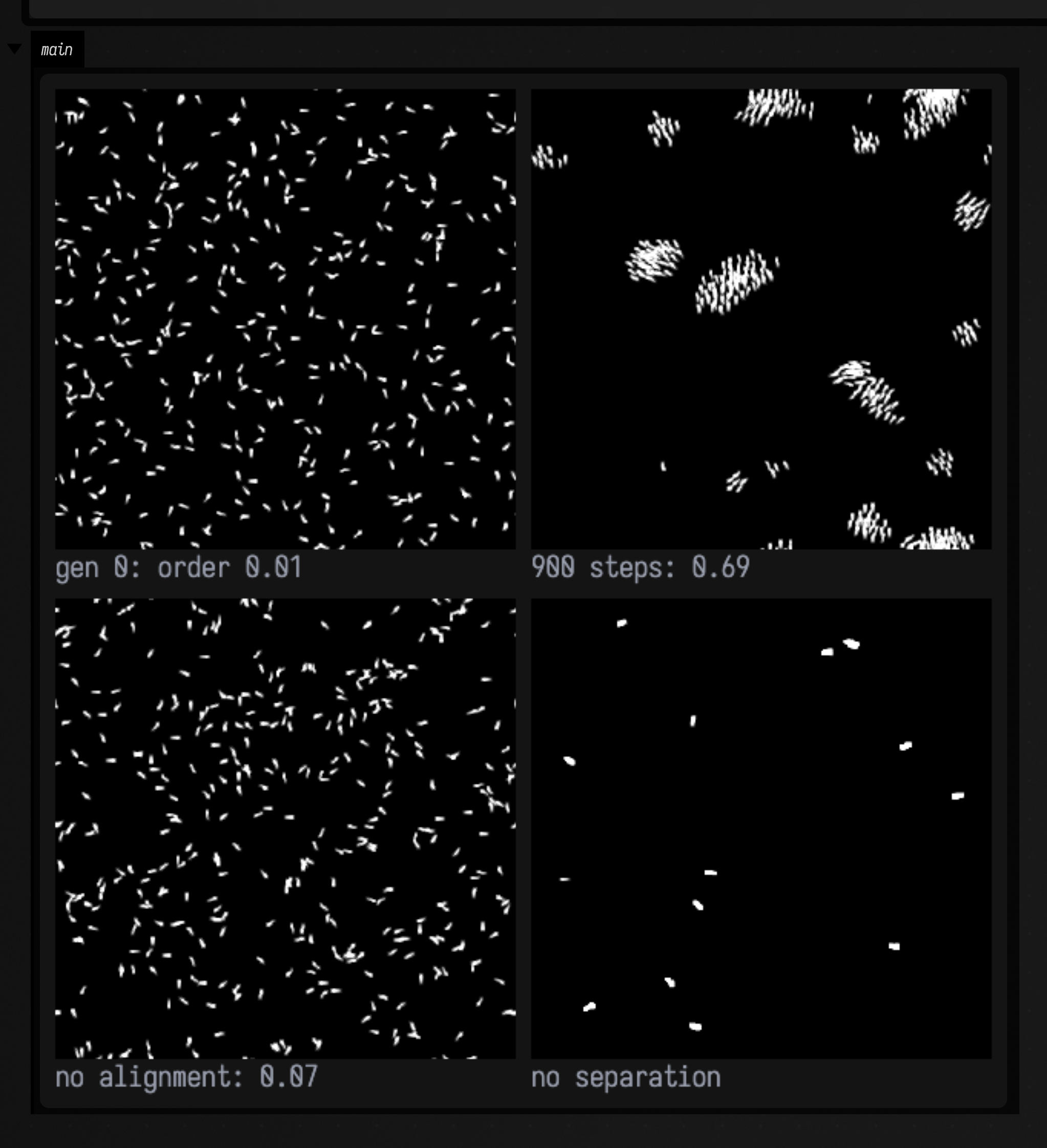

The control arm, running beside it

The two numbers above, 0.692 and 0.073, are the same initial state with one weight changed. Both panels are the identical 400 agents from the identical seed; the right one has alignmentWeight = 0 and nothing else is different. 900 steps in seven seconds, six or seven per displayed frame, with the order parameter in each caption recomputed every frame.

What to watch: the left panel's flocks are not there at the start and nobody puts them there. Within about a hundred steps local alignment has produced a handful of coherent groups, and after that the interesting event is the rare one: two flocks meeting and either merging or passing through. That is why the order parameter settles near 0.69 rather than climbing to 1: it is the global average over several flocks that each individually agree, and the caption's number wobbles as they merge and split. On the right, the population stays a gas forever. It is moving, since the speed floor is still on; it just never agrees about anything.

The tail is drawn longer here (8 units) than in the still (5) and the domain is drawn at one pixel per unit rather than 1.4. Both are frame-rate accommodations: at six or seven steps per displayed frame an agent covers about nine units between frames, so a short tail leaves visible gaps. Neither changes anything measured, because order() reads the velocity array and not the picture.

:::static
:::fold draw both populations, and measure the order parameter every frame
/*
One pixel per domain unit, with an 8-unit motion streak behind each agent -- long enough to join
up at nine units of travel per frame. `order()` reads the velocity array, so neither choice
touches what is measured; the number in each caption is computed fresh every frame.
*/
fun flocks(a: BoidFlock, b: BoidFlock, n: Int) = [
    "flock " + n + ": order " + a.order().f2 to a.toImg(1.0, tail = 8.0),
    "no align " + n + ": " + b.order().f2 to b.toImg(1.0, tail = 8.0),
]

:::endfold

/*
The same initial state, twice, stepped together -- so the ONLY difference between the two panels
is the alignment weight. 900 steps over 140 displayed frames: six or seven steps per frame, and
no ramp -- a flock's rate of change is roughly constant, which is exactly when linear is right.
*/
val params = BoidParams()
val blind = params.copy(alignmentWeight = 0.0)
val start = BoidFlock.random(400, 260.0, 260.0, speed = 1.4, seed = 4L)
animateEvolution(
    start.copy() to start.copy(),
    totalSteps = 900,
    seconds = 7.0,
    columns = 2,
    cellSide = 300,
    step = { (a, b) ->
        a.step(params)
        b.step(blind)
        a to b
    },
    panels = { (a, b), n -> flocks(a, b, n) },
)

7. Physarum

Jones' slime-mould model. Each agent deposits into a trail field, samples that field three ways ahead, turns toward the strongest, and moves. The network is not stored anywhere; it is the fixed point of that stigmergic loop.

The measurement is topShare(0.05): the fraction of all deposit held by the brightest 5 % of pixels. A flat field gives 0.05 by definition. The sensing population gives 0.480; the identical population with sensing switched off (same count, same seed, same deposit, same decay, random turns) gives 0.185. And the shapes differ as sharply: median isoperimetric ratio 17.2 against 1.2, filaments against blobs.

:::static
/*
Jones' Physarum model: agents deposit into a trail field, sense it three ways ahead, turn toward
the strongest, move. The transport network is nowhere in the code -- it is the fixed point of
that loop.

The measurement: `topShare(0.05)` is the fraction of all deposit held by the brightest 5% of
pixels. A flat field gives 0.05. A network concentrates material into filaments and gives much
more. The control is the identical population with sensing switched off -- same count, same
seed, same deposit, same decay, random turns.
*/
val side = 256
val p = PhysarumParams()
val sensing = PhysarumSwarm.disc(side, side, 6000, 0.55, seed = 6L).stepTimes(p, 400, seed = 6L)
val blind = PhysarumSwarm.disc(side, side, 6000, 0.55, seed = 6L).stepTimes(p.copy(sensing = false), 400, seed = 6L)

println(
    "top-5% deposit share: sensing " +
        sensing.trail.topShare(0.05).f3 +
        ", CONTROL sensing off " +
        blind.trail.topShare(0.05).f3 +
        " (a flat field gives 0.05)",
)
println("sensing morphology: " + sensing.trail.normalized().morphology())
println("blind   morphology: " + blind.trail.normalized().morphology())

:::fold draw both trail fields in magma
showImg(
    montage(
        [
            "sensing" to sensing.trail.normalized().colormap("magma"),
            "CONTROL: sensing off" to blind.trail.normalized().colormap("magma"),
        ],
        columns = 2,
        cellSide = 340,
    ),
)
:::endfold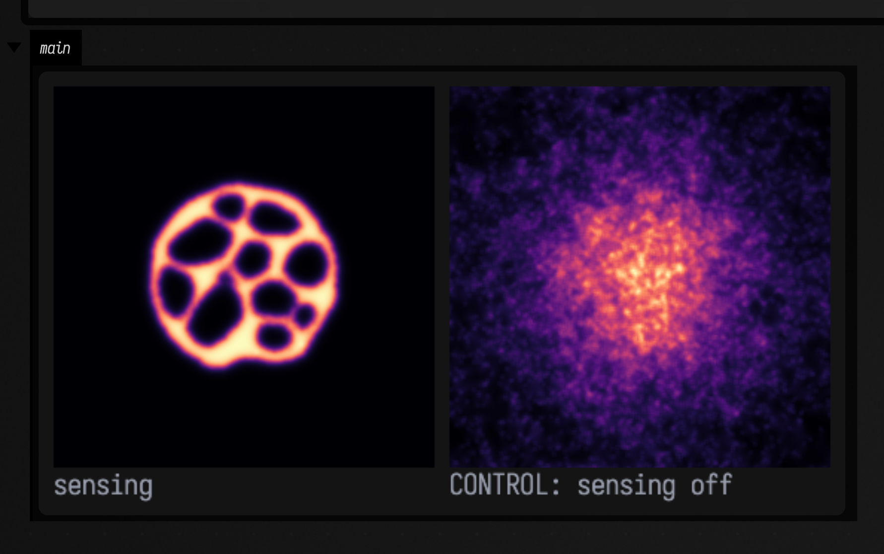

Watching the network find itself

topShare climbing from 0.05 to 0.48 is the evidence; the clip is what the number is about. 400 steps in seven seconds, three per displayed frame, both populations stepped together, with the top-5 % share recomputed and printed every frame.

Three things to watch, and the third is the one worth waiting for:

1. The disc expands, in both panels. That is not the network; that is 6000 mutually exclusive agents needing room.
2. In the sensing panel the expansion goes anisotropic almost immediately: some directions get reinforced and the rest go dark. Nothing chose those directions. They are wherever the deposit happened to be a little stronger when the agents first looked.
3. Then the interior reorganises: trails that were separate merge, and loops close and re-open. The share number keeps climbing while the shape keeps changing, because the network is a fixed point of the loop rather than something that gets built and then stops.

The blind panel is the same 6000 agents with sensing = false, so it expands and then just sits there, uniform, at a share that stays near a fifth of the sensing run's.

:::static
:::fold draw both trails on one derived colour range, and measure the share every frame
/*
Both panels on ONE derived range, not on each other's maxima: a cell an agent occupies every
step accumulates `deposit` and keeps `decay` of what it had, so it converges to
deposit / (1 - decay) = 62.5. A lower ceiling clips the network to flat cream. The caption's number is
`topShare(0.05)`, recomputed every frame.
*/
val p = PhysarumParams()
val ceiling = (p.deposit / (1.0 - p.decay)).toFloat()
fun trails(a: PhysarumSwarm, b: PhysarumSwarm, n: Int) = [
    "sensing " + n + "  " + a.trail.topShare(0.05).f3 to a.trail.colormap("magma", 0f, ceiling),
    "blind " + n + "  " + b.trail.topShare(0.05).f3 to b.trail.colormap("magma", 0f, ceiling),
]

:::endfold

/*
Sensing and blind, from the same seed, stepped together: 400 steps over 140 displayed frames,
so three deposit-sense-move rounds per frame. `step` takes its rng explicitly, so each
population gets its own stream -- exactly what `stepTimes(p, 400, seed = 6L)` does internally,
which is why these panels land on the same numbers as the figure above.
*/
val rngA = kotlin.random.Random(6L)
val rngB = kotlin.random.Random(6L)
animateEvolution(
    PhysarumSwarm.disc(256, 256, 6000, 0.55, seed = 6L) to PhysarumSwarm.disc(256, 256, 6000, 0.55, seed = 6L),
    totalSteps = 400,
    seconds = 7.0,
    columns = 2,
    cellSide = 300,
    step = { (a, b) -> a.step(p, rngA) to b.step(p.copy(sensing = false), rngB) },
    panels = { (a, b), n -> trails(a, b, n) },
)

A million agents on the GPU

The same rule runs on the GPU as ShaderPhysarumSystem: a million agents on a trail 512 pixels high, each one a single vertex-shader invocation per frame that senses, turns, steps and deposits. The defaults are the PhysarumParams defaults above. The trail is a TrailField, a stigmergy field you can use on its own: four channels, each with its own half-life, plus diffusion and wind. Any module can deposit into it, and any shader can read it with #include "trail/sample". Here there are two species, one per channel. Each follows its own trail and avoids the other's:

// 512 pixels high and as wide as the window's shape needs, so the trail is not stretched
var physarum = ShaderPhysarumSystem() {
    height = 512
    width = 512 * window.width / window.height
    agentCount = 1_000_000
    speciesCount = 2
    exposure = 0.05f
}

// steps once a frame and draws the trail, one colour per species
physarum.installInto()

A million agents scattered as noise, drawing themselves into two networks:

These agents do not exclude each other. On the GPU the density does the job that exclusion does on the CPU: at one agent per pixel, a trail that pulls in more agents also fills up. Read back after 600 frames, the trail gives topShare(0.05) = 0.75 with one species. The same agents with sensing = false give 0.065, close to the flat 0.05. The settings are read every frame, so you can change physarum.trail.settings.windPx or physarum.settings.jitter while it runs.

8. Diffusion-limited aggregation

Diffusion-limited aggregation: a seed at the centre, then particles released far away that random-walk until they touch the cluster and stick. Nothing in the rule mentions branches, and the result is a dendrite.

It is the one system in the family with a quantitative number to hit: the mass–radius dimension, fitted as N(r) ∝ r^D in log–log space by massRadiusDimension, which also reports \( r^2 \), because a slope through a curve is not a dimension. Planar DLA's asymptotic value is about 1.71; the cluster below measures 1.597 with \( r^2 = 0.9965 \).

The two controls are what make that number mean something. An Eden cluster uses the same neighbourhood and the same particle count, and differs only in that the growth site is chosen uniformly instead of by a diffusing walker: it measures 1.860 and is visibly compact. A uniform sprinkle over the same disc has dimension exactly 2 by construction and measures 1.898. So the estimator is reading the diffusion-limited part of DLA and not merely "a growth process happened", and it is not simply reading the bounded support.

:::static
/*
Diffusion-limited aggregation: a seed, then particles released far away that random-walk until
they touch and stick. Nothing in the rule mentions branches.

This is the one system here with a quantitative number to hit, so it gets the sharpest evidence:
the mass-radius dimension. An Eden cluster (same neighbourhood, growth site chosen uniformly
instead of by a diffusing walker) and a uniform sprinkle both have dimension 2, so those two
controls show the estimator is reading the diffusion-limited part and not merely "growth".
*/
val side = 300
val dla = dlaCluster(side, side, particles = 6000, seed = 2L)
val fit = dla.fractalDimension(rMin = 5.0, rMaxFraction = 0.75)
println(dla)
println("DLA mass dimension " + fit.dimension.f3 + " (r2 = " + fit.rSquared.f4 + ")")

val eden = edenCluster(side, side, particles = dla.points.size, seed = 2L)
val edenFit = eden.fractalDimension(rMin = 5.0, rMaxFraction = 0.75)
println("CONTROL Eden dimension " + edenFit.dimension.f3)
val sprinkle = sprinkleCluster(side, side, dla.points.size, dla.maxRadius, seed = 2L)
val sprinkleFit = massRadiusDimension(
    sprinkle.points,
    sprinkle.center,
    rMin = 5.0,
    rMax = sprinkle.maxRadius * 0.75,
    minCount = 60,
)
println("CONTROL uniform sprinkle dimension " + sprinkleFit.dimension.f3 + " (exactly 2 by construction)")

:::fold draw all three clusters, the first two coloured by arrival order
showImg(
    montage(
        [
            "DLA: D = " + fit.dimension.f2 to dla.arrivalOrderImg().colormap("turbo"),
            "Eden: D = " + edenFit.dimension.f2 to eden.arrivalOrderImg().colormap("turbo"),
            "sprinkle: D = " + sprinkleFit.dimension.f2 to sprinkle.mask,
        ],
        columns = 3,
        cellSide = 280,
    ),
)
:::endfold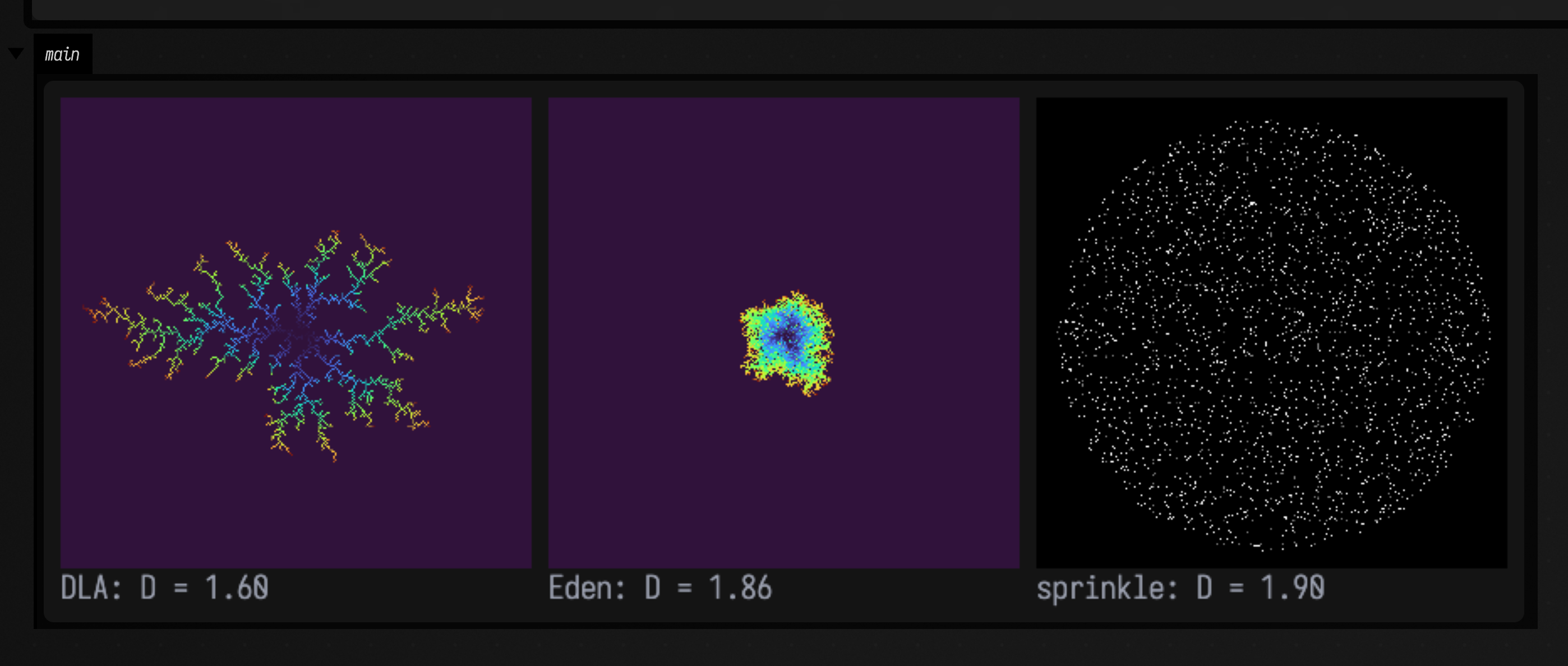

The order the branches arrived in

A DLA cluster's shape is a record of when. The cluster is grown once, by dlaCluster, and Aggregate.points is the order the particles stuck in. The clip reveals that recorded order at a uniform rate. It is not a re-simulation and it is not uniform in the original walk's wall-clock either: a late particle takes far longer to arrive than an early one, because it has to random-walk in from a larger circle past a bigger target. What is uniform is particle count.

Screening. The interior stops growing almost immediately: once a branch has neighbours on both sides, a walker arriving from outside is overwhelmingly likely to touch a tip first, so it never reaches the inside. What grows is a small number of tips racing outward while everything behind them is frozen, and that is why a mass–radius fit gives 1.6 and not 2: the interior is permanently empty, made empty by the arrival process rather than by the rule.

:::static
// Grow the cluster once, then replay `Aggregate.points` -- which IS the order the particles stuck
// in -- at a uniform rate over seven seconds.
val dla = dlaCluster(300, 300, particles = 6000, seed = 2L)

:::fold crop once to the finished cluster's bounding box, and colour by arrival order on its full scale
/*
The crop is the colour-range discipline in geometry: taken ONCE, from the finished cluster, never
from the frame -- a crop that tracked the growing prefix would zoom out as the cluster grew and
the screening this clip is about would be the one thing you could not see.

Per AXIS rather than a square around maxRadius: a DLA cluster is anisotropic, and maxRadius is set
by its single longest arm, so a square crop leaves a third of the panel permanently empty.
*/
val pad = 2
val x0 = (dla.points.minOf { it.x }.toInt() - pad).coerceAtLeast(0)
val y0 = (dla.points.minOf { it.y }.toInt() - pad).coerceAtLeast(0)
val cw = (dla.points.maxOf { it.x }.toInt() + pad + 1 - x0).coerceAtMost(300 - x0)
val ch = (dla.points.maxOf { it.y }.toInt() + pad + 1 - y0).coerceAtMost(300 - y0)

/*
`arrivalPrefixImg` fixes the colour ramp to the FULL cluster's particle count, so a branch keeps
the colour it arrived with; `arrivalOrderImg` normalises by its own count and would re-map the
newest particle to the top of turbo on every frame.
*/
fun cluster(dla: Aggregate, n: Int) = [
    "particles " + n + " of " + dla.points.size to
        dla.arrivalPrefixImg(n).crop(x0, y0, cw, ch).colormap("turbo", 0f, 1f).upscaleNearest(3),
]

:::endfold

/*
Why the crop: a cluster is a fixed amount of ink, and how legible its growth is depends entirely on
how much of the frame that ink occupies. Note the particle count in the first line -- `particles`
is a ceiling, not a promise, and this cluster stopped well short of the 6000 asked for.
*/
println(dla)
println(
    "cropped to " +
        cw +
        " x " +
        ch +
        " of 300 x 300, so " +
        (100.0 * dla.points.size / (cw * ch)).f1 +
        "% of the panel is ever lit, against " +
        (100.0 * dla.points.size / 90000.0).f1 +
        "% uncropped",
)

animateEvolution(
    Unit,
    totalSteps = dla.points.size,
    seconds = 7.0,
    cellSide = 660,
    step = { it },
    panels = { _, n -> cluster(dla, n) },
)

9. L-systems

L-systems are the odd one out in this family. They are the one generative system here whose output can be checked exactly and combinatorially.

• Lindenmayer's original algae system (A → AB, B → A) has derivation lengths that are the Fibonacci numbers. Exactly.
• The Koch snowflake has exactly \( 3 \cdot 4^n \) forward symbols at generation n.
• Its turtle path closes: the pen returns to where it started, to \( 2.3 \times 10^{-14} \) of a step.
• Its drawn length grows by exactly 4× per generation at constant step size. (The textbook 4/3 is the ratio when the figure is held at constant diameter; this turtle holds the step constant, so the figure triples in size each generation. Same identity, stated for what is actually drawn.)
• And its enclosed area matches the closed form \( 9^n \cdot A_0 \cdot \bigl(1 + \tfrac{3}{5}(1 - (4/9)^n)\bigr) \) to \( 3 \times 10^{-8} \) relative, a second independent geometric identity from the same turtle. (FLine stores single-precision coordinates; that residual is the float, not the identity.)

Perturbing the turn angle by 0.01 radians leaves the path open by 2.7 steps, so the closure test has teeth.

The bracket pair [ ] is what makes an L-system a plant rather than a curve: it pushes and pops the turtle state, so a production can grow a side branch and return. And stochastic productions (several competing rules for one symbol) vary the topology rather than jittering one plant's coordinates, which is why the three plants below have 91, 74 and 51 branches rather than three wobbly copies of the same tree.

:::static
// L-systems are the one generative system in this family whose output can be checked exactly and
// combinatorially rather than statistically -- so they carry the sharpest evidence here.
println("algae derivation lengths (Fibonacci): " + LSYSTEM_ALGAE.derivations(9).map { it.length })
println(
    "Koch snowflake forward symbols (3 * 4^n): " +
        (0..5).map { gen -> LSYSTEM_KOCH_SNOWFLAKE.derive(gen).count { it == 'F' } },
)

/*
And the turtle: the path CLOSES, its drawn length quadruples exactly at constant step size, and
its enclosed area matches the closed form 9^n * A0 * (1 + 3/5(1 - (4/9)^n)). FLine stores
single-precision coordinates, so "exact" here means to float precision.
*/
val step = 1.0
val tp = TurtleParams(angle = Math.PI / 3.0, step = step)
val gens = (0..5).map { drawLSystem(LSYSTEM_KOCH_SNOWFLAKE, it, tp) }
println("worst closure residual: " + gens.map { turtleClosureError(it, step) }.max() + " of a step")
val lens = gens.map { flineTotalLength(it.lines) }
println("length ratio per generation: " + (1..5).map { (lens[it] / lens[it - 1]).f6 })
println(
    "area, relative error against the closed form: " +
        (0..5).map { gen ->
            val a0 = Math.sqrt(3.0) / 4.0 * step * step
            val predicted =
                Math.pow(9.0, gen.toDouble()) * a0 * (1.0 + 0.6 * (1.0 - Math.pow(4.0 / 9.0, gen.toDouble())))
            "%.1e".format(Math.abs(Math.abs(flineSignedArea(gens[gen].lines)) - predicted) / predicted)
        },
)
// Control: one wrong turn and none of that holds.
println(
    "CONTROL, turn angle perturbed by 0.01 rad: open by " +
        "%.1f"
            .format(
                turtleClosureError(drawLSystem(LSYSTEM_KOCH_SNOWFLAKE, 4, tp.copy(angle = Math.PI / 3.0 + 0.01)), step),
            ) +
        " steps",
)

// Stochastic productions vary the TOPOLOGY, not merely the coordinates.
val plants = (1L..3L).map {
    drawLSystem(LSYSTEM_STOCHASTIC_PLANT, 5, TurtleParams(angle = Math.toRadians(24.0), step = 4.0), seed = it)
}
println("three seeds of the stochastic plant give branch counts " + plants.map { it.lines.size })

// The arrowhead curve draws on A and B, not F -- with the default alphabet it renders nothing.
val arrow = drawLSystem(LSYSTEM_SIERPINSKI_ARROWHEAD, 7, TurtleParams(angle = Math.PI / 3.0, drawSymbols = "AB"))
println("arrowhead, generation 7: " + arrow.drawnSegments + " drawn segments (3^7 = 2187)")

:::fold rasterize the three curves and the three plants
showImg(
    montage(
        [
            "Koch snowflake gen 4" to rasterizeFLines(gens[4].lines, 300, 300),
            "arrowhead gen 7" to rasterizeFLines(arrow.lines, 300, 300),
            "dragon gen 12" to
                rasterizeFLines(drawLSystem(LSYSTEM_DRAGON, 12, TurtleParams(angle = Math.PI / 2.0)).lines, 300, 300),
        ] + plants.mapIndexed { i, pl -> "plant seed " + (i + 1) to rasterizeFLines(pl.lines, 240, 300) },
        columns = 3,
        cellSide = 280,
    ),
)
:::endfold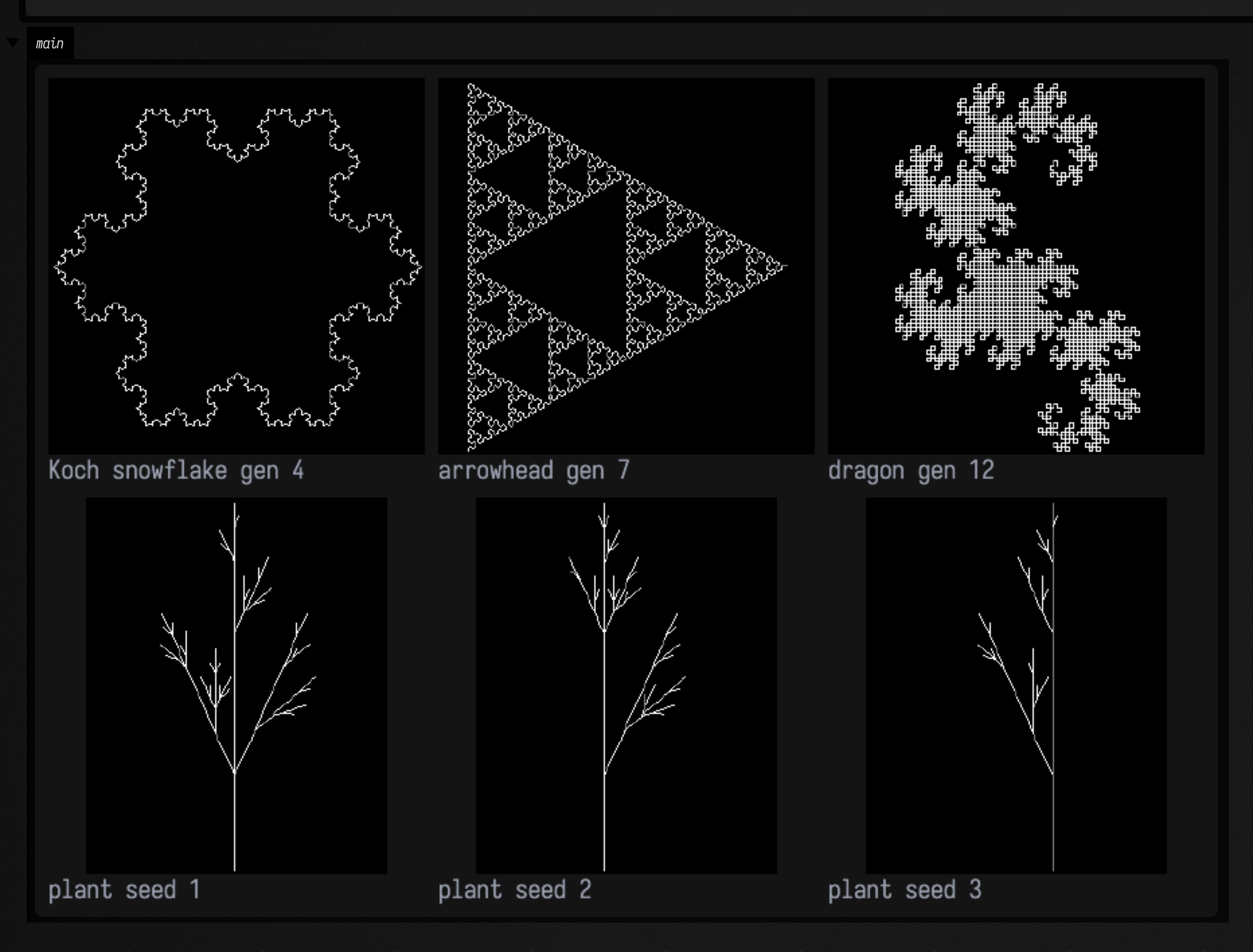

The turtle, walking

An L-system could be animated by derivation depth, generation 0 then 1 then 2, and that would be a slideshow: six generations over seven seconds is 23 duplicate frames between each change, and each generation is a completely different picture, so there is no motion to read, only cuts.

What an L-system does have is a turtle, and a turtle walks in an order. flinePrefix truncates the emitted FLines at a fraction of their total segment count in walk order, so both panels below are drawn by a pen, in the sequence the pen moved.

Which makes the bracket pair visible in the right-hand panel. [ pushes the turtle's state and ] pops it, so a plant is drawn depth-first: the pen runs all the way out to the tip of one branch, then jumps back to a fork it remembered and runs out to the next. You can watch it do exactly that, and the jumps are the stack. The Koch snowflake on the left has no brackets at all and is therefore one continuous stroke: 768 segments at generation 4, traced without the pen ever leaving the paper, closing back on its start to \( 2.3 \times 10^{-14} \) of a step.

:::static
:::fold rasterize each prefix in the finished curve's frame
/*
`rasterizeFLinesFramed` takes its framing from the FINISHED curve. Plain `rasterizeFLines` fits
the raster to whatever it is handed, so a growing prefix rescales every frame: the curve appears
to stay the same size while the world shrinks around it, and the growth becomes invisible.
*/
fun drawn(koch: List<FLine>, plant: List<FLine>, f: Double): List<Pair<String, Img>> {
    val pct = (f * 100).toInt()
    return [
        "Koch gen 4: " + pct + "% drawn" to rasterizeFLinesFramed(flinePrefix(koch, f), koch, 420, 420),
        "plant gen 5: " + pct + "% drawn" to rasterizeFLinesFramed(flinePrefix(plant, f), plant, 420, 420),
    ]
}

:::endfold

/*
Animated by DRAWING, not by cutting between derivation depths: an L-system's turtle walks in an
order, and `flinePrefix` truncates the emitted FLines at a fraction of their segment count in
exactly that order. 240 ticks over 140 displayed frames.
*/
val koch = drawLSystem(LSYSTEM_KOCH_SNOWFLAKE, 4, TurtleParams(angle = Math.PI / 3.0, step = 1.0))
val plant = drawLSystem(LSYSTEM_STOCHASTIC_PLANT, 5, TurtleParams(angle = Math.toRadians(24.0), step = 4.0), seed = 1L)
val ticks = 240
animateEvolution(
    Unit,
    totalSteps = ticks,
    seconds = 7.0,
    columns = 2,
    cellSide = 420,
    step = { it },
    panels = { _, n -> drawn(koch.lines, plant.lines, n.toDouble() / ticks) },
)

10. Bridges out: FLines, trees and a watertight mesh

What makes this family Field's rather than a generic ALife library is where its output goes. Three bridges, all into machinery that was already here:

1. A reaction–diffusion field → FLines. Img.isoContourFLines runs the marching-squares extractor in contours.kt over the v field, so a Gray–Scott result becomes drawable, animatable, exportable geometry: 195 contours at v = 0.25 below. That count is checked against a second measurement rather than printed: CI asserts at least one loop per thresholded blob, and pins the extractor itself against circle geometry (a disc's contour encloses \( \pi r^2 \) to 0.16 %).
2. Space colonization → a tree of FLines. Grown into an annulus, which no upward-with-noise heuristic reaches, so the branching really is following the space. ColonizationTree.isTree() checks the thing a picture cannot show (one root, \( n - 1 \) edges, no cycles) because a growth algorithm that produces a cycle looks identical.
3. A 3-D life-like automaton → a TriMesh. IntVolume.toMesh smooths the occupancy and runs mesh_sdf.kt's marching cubes, so the automaton's surface is a real mesh you can boolean, subdivide and export. The claim asserted is that it is watertight: a leaking mesher produces a picture that looks fine and a model that cannot be printed.

:::static
/*
What makes this family Field's rather than a generic ALife library: the bridges out into the
things Field already draws, meshes and exports.

(a) A reaction-diffusion field -> iso-contour FLines, through the marching-squares extractor in
    `contours.kt` that was already here.
*/
val rd = grayScottSeed(96, 96, patches = 5, patchSize = 12, seed = 4L).stepTimes(GRAY_SCOTT_SPOTS, 5000)
val contours = rd.v.isoContourFLines(0.25, cells = 96)
println("Gray-Scott -> " + contours.size + " iso-contour FLine(s) at v = 0.25")

/*
(b) Space colonization -> a tree of FLines. Grown into an ANNULUS, which no upward-with-noise
    heuristic reaches, so the branching really is following the space. isTree() checks the thing
    a picture cannot show: one root, n-1 edges, no cycles.
*/
val ring = annulusAttractors(1400, 150.0, 140.0, 60.0, 120.0, seed = 3L)
val tree = spaceColonization(ring, 150.0, 285.0, influenceRadius = 30.0, killRadius = 7.0, stepSize = 5.0)
println(tree)
println("is a tree (one root, n-1 edges, acyclic): " + tree.isTree())
println("CONTROL, no attractors: " + spaceColonization(emptyList(), 150.0, 285.0).nodeCount + " nodes")

/*
(c) A 3-D life-like automaton -> a TriMesh, through `mesh_sdf.kt`'s marching cubes. The claim
    that matters for a mesh is that it is WATERTIGHT -- a leaking mesher looks fine and produces
    a model that cannot be printed, booleaned or subdivided. Note an EMPTY mesh is vacuously
    watertight, so the triangle count is part of the claim.
*/
val volume =
    IntVolume.randomBall(48, 48, 48, density = 0.55, ballFraction = 0.70, seed = 8L).stepTimes(LIFE3D_CLOUDS, 6)
println(volume)
val mesh = volume.toMesh(resolution = 96, smoothRadius = 1)
println(
    "marched: " +
        mesh.triangleCount +
        " triangles, watertight = " +
        mesh.isWatertight() +
        ", Euler characteristic = " +
        mesh.eulerCharacteristic(),
)

:::fold draw the field, the contours, the tree and two views of the volume
showImg(
    montage(
        [
            "Gray-Scott field" to rd.v.colormap("magma", 0f, 0.5f).upscaleNearest(3),
            "its iso-contours as FLines" to rasterizeFLines(contours, 300, 300),
            "space colonization tree" to rasterizeFLines(tree.toFLines(), 300, 300),
            "3-D CA: z slice" to volume.slice(24).toImg(2).upscaleNearest(5),
            "3-D CA: depth projection" to volume.depthProjection().colormap("viridis").upscaleNearest(5),
        ],
        columns = 3,
        cellSide = 280,
    ),
)
:::endfold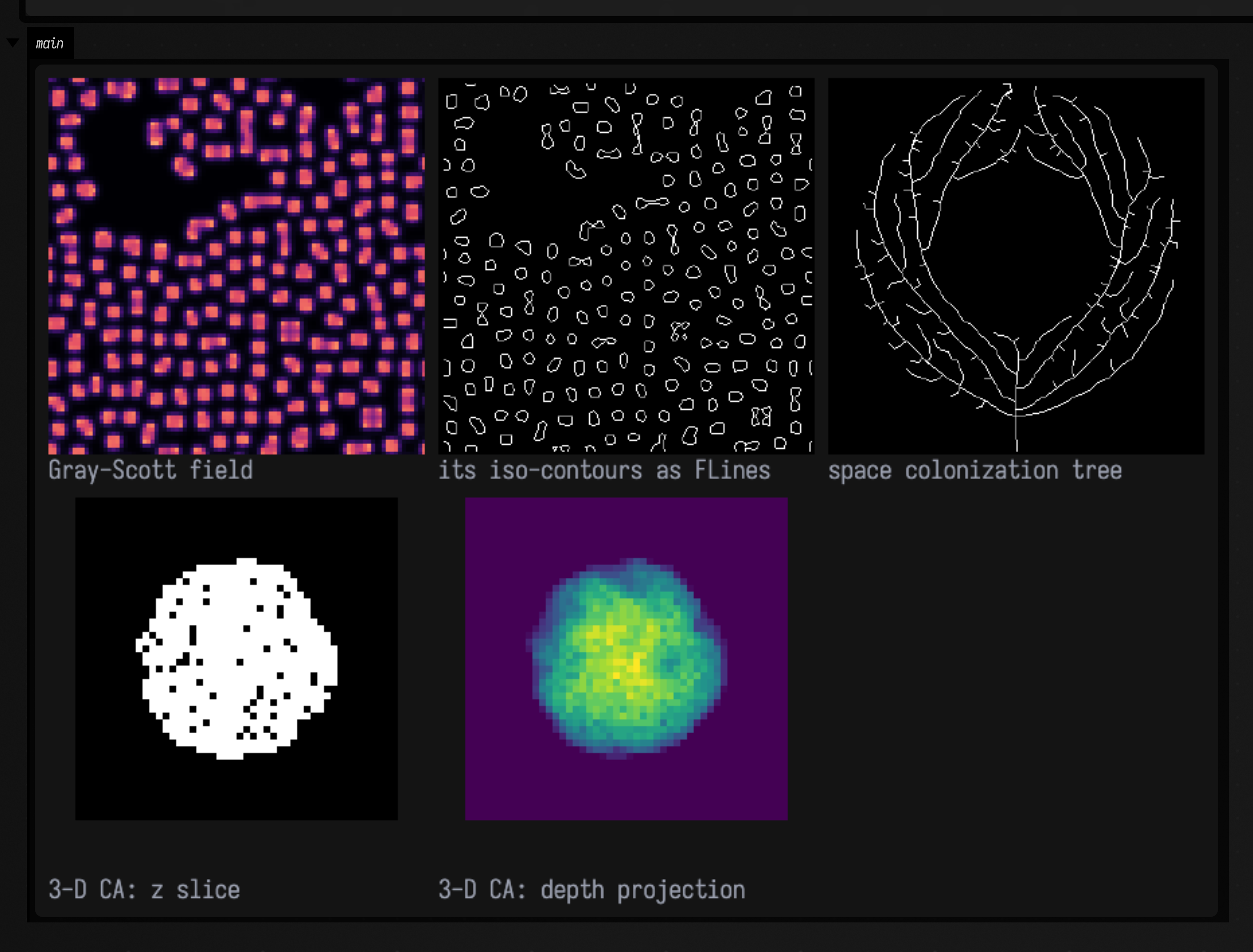

The bridge, live: a field and its contours at the same time

The first of those three bridges is the one worth animating, because it is the one that produces geometry rather than a picture, and geometry that tracks a moving field is the thing you would actually want in a Field document. Left: the v field of a spots run, 5000 steps in seven seconds. Right: the same field's v = 0.25 iso-contours, re-extracted every frame through contours.kt's marching squares, with the loop count in the caption.

The loop count climbs while the spots are dividing, because each division is one loop becoming two, and it is the one number on this page that is a topological measurement rather than a statistical one: it changes by integers, at the moment a thing happens. The contours stay locked to the field's level set as it moves.

:::static
:::fold pin the contour panel's framing to the field's extent
/*
The contour panel is framed by the FIELD's extent -- two invisible single-node FLines at the
corners of the 96x96 sample grid, in the contour extractor's own pixel coordinates. Framed by
the contours' own bounds instead, the early frames (two loops in one corner) would be drawn
zoomed right in and the whole figure would zoom out as the pattern spread.
*/
val fieldFrame = [FLine().moveTo(0, 0), FLine().moveTo(95, 95)]
fun bridge(s: GrayScottState, n: Int): List<Pair<String, Img>> {
    val loops = s.v.isoContourFLines(0.25, cells = 96)
    return [
        "v field, step " + n to s.v.colormap("magma", 0f, 0.5f).upscaleNearest(4),
        "iso v=0.25: " + loops.size + " loops" to rasterizeFLinesFramed(loops, fieldFrame, 384, 384),
    ]
}

:::endfold

/*
A reaction-diffusion field and its iso-contour FLines, re-extracted afresh every frame -- so the
geometry tracks the field instead of being a snapshot of it. 5000 steps over 140 displayed
frames: 36 reaction-diffusion steps AND one marching-squares pass per frame.
*/
animateEvolution(
    grayScottSeed(96, 96, patches = 5, patchSize = 12, seed = 4L),
    totalSteps = 5000,
    seconds = 7.0,
    columns = 2,
    cellSide = 384,
    step = { it.step(GRAY_SCOTT_SPOTS) },
    panels = { s, n -> bridge(s, n) },
)

11. Evolution: searching the rule space

Every section above picks a rule and measures what it does. This one runs the question backwards: given a measurement, find a rule that scores well on it.

The statistics the sections above measure with are the fitness functions this one searches on: alife.kt's polarization, blobShapes, correlationLength, massRadiusDimension, stateEntropyBits and centroidDrift, read as a score instead of as a readout.

Each search is compared with a control, PopulationSearch.random. It draws from exactly the distribution evolve mutates within, at the same budget, under the same seed, and every result below is a margin over it. Without it the numbers would mean nothing: a generator good enough to stumble onto a decent rule now and then looks identical, from the outside, to a search that works.

A Lenia rule that travels

A soliton, meaning alive and in one piece and moving, is the thing continuous Lenia is famous for, and it is three measurements Field already had. Every term of the score is read off leniaRun, which classifies a run as DEATH, BOUNDED or SATURATION from the mean field value and reports a wrapped centroid drift. That matters because the failure mode here is a rule that scores well by saturating the grid and sitting still.

Against 220 evaluations of the control at the same seed, evolution finds a rule 17.2 % better: 2.09372 against 1.78636, a margin of 0.3074. The first panel of the figure below is the control's best, so the thing evolution had to beat is in the same picture at the same budget.

The search scored what it was asked to score, and that is less than a creature. At the 90 steps the objective runs, the evolved rule is BOUNDED with one blob and a centroid drift of 4.82 cells: the smooth ring in the last panel. Run the same rule from the same seed for 300 steps and it has broken into 14 blobs with a mean field of 0.32, so what evolution found is a ring on its way to filling the board. Orbium, by contrast, holds its mass level for as long as you run it. To search for creatures, score a longer run, or score how little the mass changes over its second half.

:::static
// Ask for a soliton: alive, in ONE piece, and travelling. Every term is read off leniaRun, which
// already classifies a run DEATH / BOUNDED / SATURATION and already reports a wrapped centroid drift.
val ops = LeniaGenome(radius = 6, dt = 0.1, shells = 3)
val objective = leniaSolitonObjective(width = 48, height = 48, steps = 90, initialSeed = 5L, driftScale = 8.0)
val budget = 220

// The control arm: the same distribution evolve mutates within, same budget, same seed.
val control = PopulationSearch.random(ops, objective, budget, seed = 13L, label = "random")
val evolved = PopulationSearch.evolve(
    ops,
    objective,
    budget,
    seed = 13L,
    mu = 6,
    lambda = 12,
    crossoverRate = 0.3,
    immigrantRate = 0.08,
    label = "evolve",
)
println(control.summary())
println(evolved.summary())
println(
    "margin %.4f  (%.1f%% above the control)"
        .format(
            evolved.bestFitness - control.bestFitness,
            100.0 * (evolved.bestFitness / control.bestFitness - 1.0),
        ),
)

val best = evolved.best!!.genome
println("evolved rule: mu=%.4f sigma=%.4f".format(best.mu, best.sigma))
println("  at 90 steps:  " + leniaRun(leniaSeed(48, 48, best, seed = 5L), best, steps = 90, sampleEvery = 8))
println("  at 300 steps: " + leniaRun(leniaSeed(48, 48, best, seed = 5L), best, steps = 300, sampleEvery = 8))

:::fold the control's best, then each successive record holder
val panels = mutableListOf<Pair<String, Img>>()
val cRule = control.best!!.genome
panels +=
    "rnd %.2f".format(control.bestFitness) to
        leniaRun(leniaSeed(48, 48, cRule, seed = 5L), cRule, steps = 90, sampleEvery = 8).field.upscaleNearest(3)
// Keep the full measured history; display at most five roughly evenly spaced record holders.
val picks =
    evolved.improvements.indices.toList().let { idx ->
        if (idx.size <= 5) idx else (1..5).map { (it * idx.size / 5) - 1 }
    }
for (i in picks) {
    val imp = evolved.improvements[i]
    panels +=
        "g%d %.2f".format(imp.generation, imp.fitness) to
            leniaRun(leniaSeed(48, 48, imp.genome, seed = 5L), imp.genome, steps = 90, sampleEvery = 8)
                .field
                .upscaleNearest(3)
}
// A FIXED 0..1 range, for the reason section "Evaluating one of these in a box" gives: a saturated
// Lenia field is constant at 1, and an auto-ranged colour map draws a constant field BLACK.
showImg(
    montage(panels, columns = 3, cellSide = 200, displayRange = 0f..1f),
    caption = "left to right: the random control's best, then each successive record holder",
)
:::endfold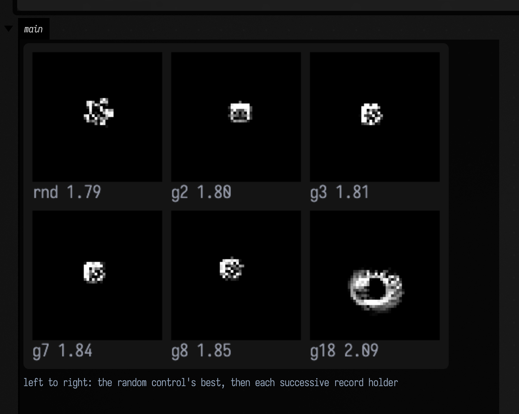

The same engine, a genome with nothing in common

A life-like rule is a table: which neighbour counts cause a birth, which cause survival. At radius 2 that is 24 birth bits and 25 survival bits: a fixed-length bit string, and therefore a genome two parents can be recombined across. LifeRuleGenome.crossover is uniform crossover over the rule table: real recombination rather than a graft.

The radius decides whether evolution has anything to do. At radius 1 the rule space is 2¹⁷, a few hundred independent draws land near the optimum on their own, and evolution wins by only 3 %. At radius 2 the space is 2⁴⁹ and the margin is 27.4 %, 0.54436 against 0.42744. A control arm that nearly wins is telling you the problem is easy rather than that the search is good, so run the control arm at whatever radius you pick.

The figure below reads oddly until you notice what the first panel is. The control is the best of 400 independent draws, so it is a high bar early on: the evolved run's first two record holders score 0.336 and 0.398 below the control's 0.427, and only overtake it around generation five. A population that started above its own control would mean the control was weak, not that the search was strong.

Selection is lexicase rather than tournament, because this objective genuinely has a case structure: one case per soup. A rule that holds together on one initial condition and collapses on the other is exactly what an average hides, and lexicase never averages.

:::static
/*
The same engine, a completely different genome.

A life-like rule is a TABLE: which neighbour counts cause a birth, which cause survival. At a
radius-2 neighbourhood that is 24 birth bits and 25 survival bits, a fixed-length bit string, and
therefore a genome two parents can be recombined across. LifeRuleGenome.crossover is uniform
crossover over the rule table: real recombination, not a graft.

Radius 2 rather than the classic Moore 8 is a deliberate choice and it is the most useful thing
in this box. At radius 1 the space is 2^17 rules, and a few hundred INDEPENDENT draws land close
to the optimum on their own, and evolution beats them by only about 3%. A control arm that nearly wins is telling you
the problem is easy, not
that the search is good. At radius 2 the space is 2^49 and the margin is 27%.
*/

val ops = LifeRuleGenome(radius = 2)
val soups = [
    randomSoup(48, 48, density = 0.35, seed = 101L),
    randomSoup(48, 48, density = 0.12, seed = 202L),
]

/*
"Alive but not saturated, and still changing" -- activity times a Gaussian band on density.
Each factor alone is trivially gamed. A rule that fills the grid and stays filled scores 1 on
density and 0 on activity; a rule that flickers every cell scores ~1 on activity and ~0 on the
band; an extinct rule scores the floor. Only the product is large for a rule that keeps a
moderate population AND keeps rearranging it, which is what everybody means by an interesting
rule and what nobody can state by looking.
*/
val objective = caEdgeOfChaosObjective(soups, warmup = 20, scored = 30)
val budget = 400

val control = PopulationSearch.random(ops, objective, budget, seed = 7L, label = "random")

/*
LEXICASE, because this objective genuinely has a case structure: one case per soup. A rule that
holds together on one initial condition and collapses on the other is exactly what a
tournament's average hides, and lexicase never averages.
*/
val evolved = PopulationSearch.evolve(
    ops,
    objective,
    budget,
    seed = 7L,
    mu = 8,
    lambda = 16,
    selection = Selection.LEXICASE,
    crossoverRate = 0.3,
    immigrantRate = 0.1,
    label = "evolve",
)

println(control.summary())
println(evolved.summary())
println()
println(
    "margin %.4f  (%.1f%% above the control)"
        .format(
            evolved.bestFitness - control.bestFitness,
            100.0 * (evolved.bestFitness / control.bestFitness - 1.0),
        ),
)
println("recombined ${evolved.recombined} children by uniform crossover over the rule table")
println()
println("evolved rule ${lifeRuleSignature(evolved.best!!.genome)}")
println("control rule ${lifeRuleSignature(control.best!!.genome)}")
println()
println("The first record holders score BELOW the control: the control is the best of 400")
println("independent draws, so a population starts under it and has to climb past it.")
println()
println("Try Selection.TOURNAMENT above and compare. Try LifeRuleGenome() with no radius argument")
println("and watch the margin collapse -- that is the easy problem, and it is worth seeing.")

:::fold the control's best, then each successive record holder, on the same soup
val panels = mutableListOf<Pair<String, Img>>()
panels +=
    "rnd %.3f".format(control.bestFitness) to
        caRun(soups[0], control.best!!.genome, 20, 30).finalGrid.toImg(2).upscaleNearest(3)
// Keep the full measured history; display at most five roughly evenly spaced record holders.
val picks =
    evolved.improvements.indices.toList().let { idx ->
        if (idx.size <= 5) idx else (1..5).map { (it * idx.size / 5) - 1 }
    }
for (i in picks) {
    val imp = evolved.improvements[i]
    panels +=
        "g%d %.3f".format(imp.generation, imp.fitness) to
            caRun(soups[0], imp.genome, 20, 30).finalGrid.toImg(2).upscaleNearest(3)
}
showImg(
    montage(panels, columns = 3, cellSide = 200),
    caption =
        "the control's best, then each successive record holder, all on the same soup -- the\n        early ones score BELOW the control, which is what overtaking looks like",
)
:::endfold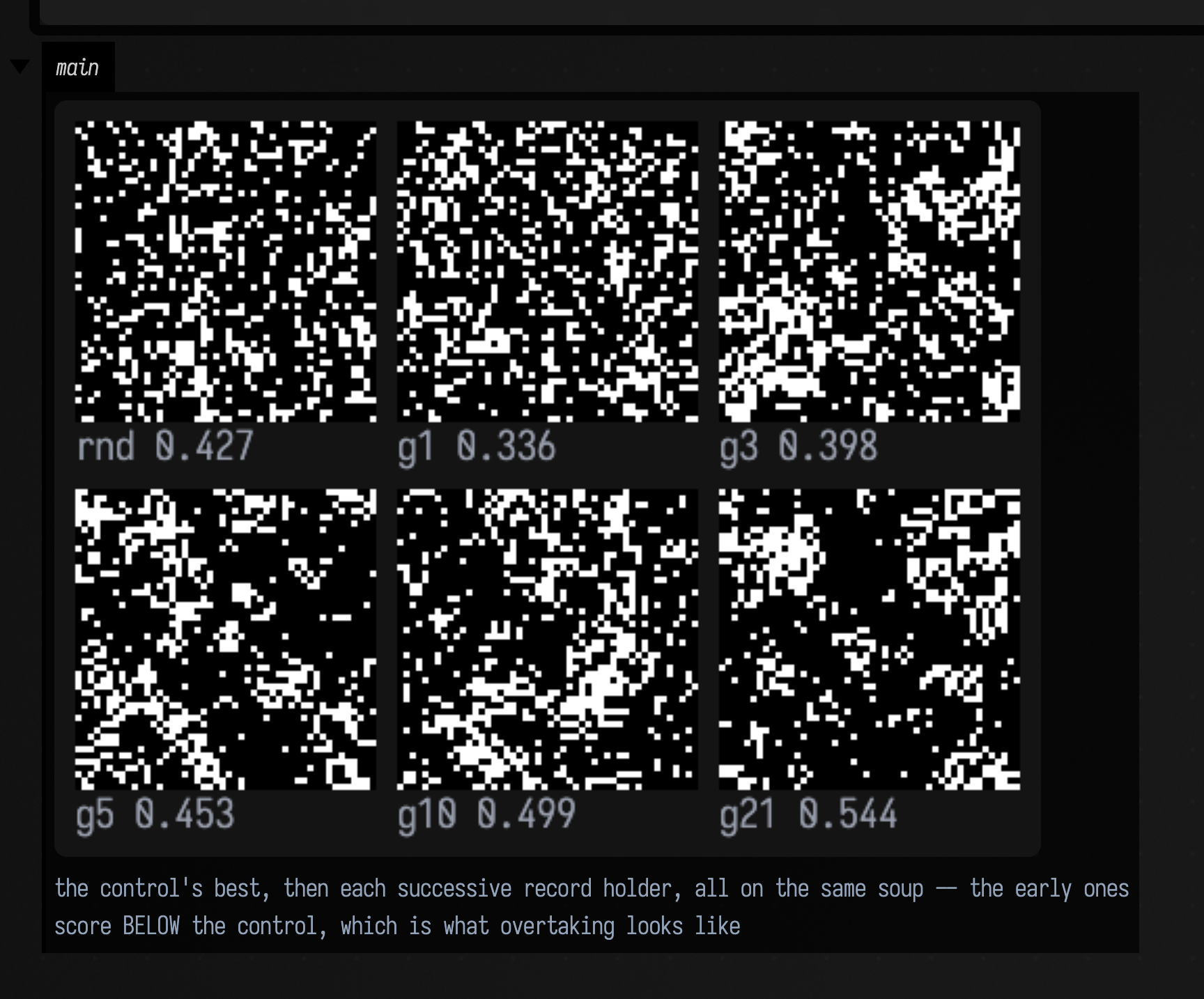

Illuminating the space instead of optimising it

MAP-Elites keeps the best rule found in each cell of a grid over the behaviour space: here (density, activity), the two numbers caEdgeOfChaosObjective already reports. What comes out is not one answer but a map of "the best rule that behaves like this".

:::static
/*
Illuminate the rule space instead of optimising it.

MAP-Elites keeps the best rule found in each cell of a grid over the BEHAVIOUR space -- here
(density, activity), the same two numbers caEdgeOfChaosObjective already reports as its
Evaluation.behaviour. What comes out is not one answer but a map of "the best rule that behaves
like THIS", which is the contact sheet below.

This is the figure worth looking at. Top left is sparse and nearly dead; bottom right is dense
and noisy; and somewhere in the middle band are the rules that hold structure while still moving.
*/

val ops = LifeRuleGenome(radius = 2)
val soups = [randomSoup(48, 48, density = 0.35, seed = 303L)]
val objective = caEdgeOfChaosObjective(soups, warmup = 20, scored = 25)
val bins = [6, 6]
val axes = [0.0..1.0, 0.0..0.6]
val budget = 600

val archive = PopulationSearch.mapElites(ops, objective, budget, axes, bins, seed = 31L, initial = 40)
println(archive)
println("off-grid (clamped to an edge cell): ${archive.offGridCandidates} of $budget")
println()

/*
The control arm for a quality-diversity claim is the same budget of independent draws, binned
identically and reduced to the best genome per cell. Comparing against a single best random rule
would be the wrong control, because MAP-Elites is not trying to find one good rule.
*/
val controlCells = HashMap<List<Int>, Double>()
val rng = kotlin.random.Random(31L)
repeat(budget) {
    val e = objective.evaluate(ops.random(rng))
    val cell =
        axes.indices.map { d ->
            (((e.behaviour[d] - axes[d].start) / (axes[d].endInclusive - axes[d].start)) * bins[d])
                .toInt()
                .coerceIn(0, bins[d] - 1)
        }
    val incumbent = controlCells[cell]
    if (incumbent == null || e.fitness > incumbent) controlCells[cell] = e.fitness
}
val controlQd = controlCells.values.sum()
println("random-sampled archive: ${controlCells.size}/${archive.cells} cells, QD %.3f".format(controlQd))
println("illuminated archive:    ${archive.elites.size}/${archive.cells} cells, QD %.3f".format(archive.qdScore))
println()
println("Quality, not coverage, is the claim. Random sampling spreads over a descriptor space for")
println("free -- that is what random means -- while MAP-Elites reaches a new cell only when a")
println("mutation moves a descriptor across a bin boundary. What illumination buys is the quality")
println("held in each cell it does occupy.")

:::fold one panel per occupied cell, labelled (density bin)(activity bin) and score
val panels =
    archive.elites.entries.sortedWith(compareBy({ it.key[0] }, { it.key[1] })).map { (cell, elite) ->
        "%d%d %.2f".format(cell[0], cell[1], elite.fitness) to
            caRun(soups[0], elite.genome, 20, 25).finalGrid.toImg(2).upscaleNearest(3)
    }
showImg(
    montage(panels, columns = 6, cellSide = 150),
    caption = "one panel per occupied cell; the label is (density bin)(activity bin) and the score",
)
:::endfold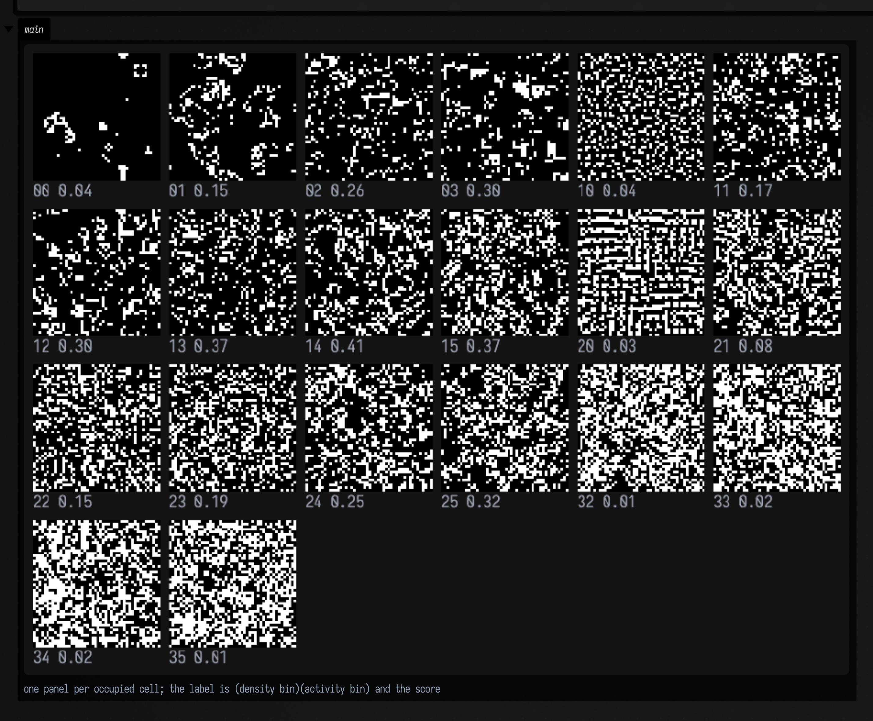

All three searches run on one engine, PopulationSearch, and each is a genome (a GenomeOps: how to make, mutate and recombine one) plus an Objective that scores it. Evolving the shape of a function for animation runs on the same engine; see evolving and optimizing functions.

Does search beat random?

One seed of evolution beside one seed of random sampling says little: the gap between two seeds of the same method is often larger than the gap between the methods. compareSearch runs every method on the same genome and objective for exactly the same number of evaluations, at many seeds, and reports the spread. Its four default arms are random sampling, a restarting hill climber, (µ6 + λ12) evolution, and (µ12 + λ24) evolution where a quarter of each generation are fresh random draws ("immigrants"). Any GenomeOps and Objective will do:

val soups = [randomSoup(48, 48, density = 0.35, seed = 101L), randomSoup(48, 48, density = 0.12, seed = 202L)]
val c = compareSearch(
    LifeRuleGenome(radius = 2),
    caEdgeOfChaosObjective(soups, warmup = 20, scored = 30),
    budget = 120,
    seeds = [1L, 2L, 3L, 4L],
    label = "life rule, edge of chaos",
)
println(c.table() + c.budgetTable([30, 60, 120]))
showImg(c.plot(360, 260))

table() gives each arm's median, interquartile range and range of per-seed bests, and how many seeds it beat random at. budgetTable reads the same runs at smaller budgets, which gives the same numbers as running those budgets separately. plot draws each arm's median best-so-far as a line with its interquartile band: random in grey, hill climbing blue, evolution orange, immigrants green. SearchArm builds other arms, and the first arm in the list is the one the others are counted against.

At 1000 evaluations and 12 seeds per arm, on the three genomes this section uses (medians of the per-seed best; in brackets, the seeds out of 12 where the arm beat random):

                      evals  random   hillclimb      evolve         immigrants
life rule, edge of    100    0.412    0.423 (7)      0.458 (9)      0.429 (5)
  chaos               300    0.426    0.470 (9)      0.486 (9)      0.470 (9)
                      1000   0.481    0.483 (7)      0.491 (6)      0.498 (8)
lenia, soliton        100    1.686    1.673 (6)      1.645 (5)      1.715 (8)
                      300    1.790    1.919 (9)      1.747 (4)      1.907 (8)
                      1000   1.899    2.197 (11)     2.037 (8)      2.135 (8)
l-system,             100    0.239    0.240 (6)      0.237 (7)      0.241 (6)
  dimension 1.7       300    0.242    0.245 (10)     0.246 (10)     0.247 (9)
                      1000   0.247    0.247 (6)      0.248 (8)      0.247 (7)

Searching helps on Lenia, and the hill climber helps most: at 1000 evaluations it beats random at 11 of 12 seeds, and three arms reach the objective's ceiling of 2.5 at their best seed. Plain evolution loses to random at 300 evaluations on Lenia and catches up only later. On Life-like rules every arm edges out random by a small median margin, but the spread is wide: random's upper quartile (0.58) is above every searcher's median, and one or two seeds of each searcher find a rule scoring above 0.95 that random never does. The L-system objective is saturated: every arm, random included, sits within 0.002 of 0.25, its practical ceiling (an exact dimension plus the straightness bonus), so this objective cannot tell the methods apart. A harder target or a finer score would be needed before it could. The vehicle brains of Braitenberg vehicles §10 run through the same compareSearch.

12. Agents with their own programs

Every system above moves its whole population with one rule: BoidFlock.step(p) applies the same parameters to every agent on every tick. ScriptWorld gives each agent a program of its own instead, written as an ordinary Kotlin function that runs on the world's clock, so one agent can circle for four seconds, head for the middle and then wander off, and the code says so in that order. The same file adds walls, and a planner for getting round them.

The clip below uses both. Twelve agents start at the left of a room divided by two walls, and each has to reach the green ring at the right. The only way through is an S: over the top of the first wall, then under the second. In the left room each agent plans a path with route(goal); in the right room each one heads straight at the goal with seek(goal). Both rooms also run avoidWalls, so the right room has good local steering, and its agents still end up pressed against the first wall, which is the part of the room nearest the goal.

:::static
// Twelve agents, one goal, two walls. The way through is an S: over the first wall, under the second.
fun maze(routed: Boolean) =
    ScriptWorld(width = 200.0, height = 200.0, seed = 1L, wrap = false).also { w ->
        w.addWall(70.0, 45.0, 70.0, 200.0, name = "gap above")
        w.addWall(130.0, 0.0, 130.0, 155.0, name = "gap below")
        val jitter = kotlin.random.Random(1L) // the same start positions in both rooms
        repeat(12) {
            w.spawn(
                18.0 + jitter.nextDouble(-8.0, 8.0),
                100.0 + jitter.nextDouble(-28.0, 28.0),
                maxSpeed = 35.0,
                radius = 1.2,
                steerResponse = 0.3,
            ) {
                val goal = point(175.0, 100.0)
                moveUntil(maxSeconds = 30.0, speed = 35.0, until = { near(goal, 6.0) }) {
                    // The one line that differs between the two rooms.
                    if (routed) route(goal, clearance = 3.5) else seek(goal)
                    avoidWalls(clearance = 3.0, weight = 0.6)
                    separate(range = 4.0, weight = 0.4)
                }
            }
        }
    }

:::fold draw both rooms, and count the agents inside the goal ring
fun arrived(w: ScriptWorld) = w.actors.count { it.distanceTo(175.0, 100.0) <= 6.0 }

fun rooms(a: ScriptWorld, b: ScriptWorld) = [
    "route %4.1f s: %d/12 in".format(a.time, arrived(a)) to a.toImg(2.0, marks = [175.0 to 100.0]),
    "seek %4.1f s: %d/12 in".format(b.time, arrived(b)) to b.toImg(2.0, marks = [175.0 to 100.0]),
]

:::endfold

// 30 simulated seconds (1800 ticks at 60 Hz), played in seven.
animateEvolution(
    maze(routed = true) to maze(routed = false),
    totalSteps = 1800,
    seconds = 7.0,
    columns = 2,
    cellSide = 400,
    step = { (a, b) ->
        a.step()
        b.step()
        a to b
    },
    panels = { (a, b), _ -> rooms(a, b) },
)

seek points at the goal and keeps pushing; avoidWalls and separate only react to what is within a few units. Deciding to go away from the goal for a while, to get round a wall, needs a plan. NavGrid makes one: an A* search on a grid where every wall is thickened by the agent's clearance, shortened by cutting corners wherever the straight line is clear, then followed waypoint by waypoint. route(goal) is that plan used as a steering term. Over 96 agents per room (8 different start layouts of 12), 0.990 of the routed agents arrive within 30 seconds and none of the direct ones do.

One agent's program

An agent's program is built from a few blocks that nest: forever, phase(name) to label a stretch of it, moveFor(seconds) to steer for a while, and parallel to run two things at once. Inside moveFor, steering terms such as orbit, arrive, wander and avoidEdges add together, so a phase can combine several. point, actor and nearest give them something to steer at.

This agent circles the centre for four seconds, closes in on it for two, and wanders for three, over and over. The caption shows the phase it is in, and the small ring is the centre it is circling.

:::static
val w = ScriptWorld(width = 200.0, height = 200.0, seed = 1L, wrap = false)
w.spawn(100.0, 40.0, maxSpeed = 45.0, radius = 1.5) {
    val centre = point(100.0, 100.0)
    forever {
        phase("orbit") { moveFor(4.0) { orbit(centre, distance = 42.0) } }
        phase("close in") { moveFor(2.0) { arrive(centre, slowRadius = 20.0) } }
        phase("wander") {
            moveFor(3.0) {
                wander(turn = 40.0)
                avoidEdges(margin = 18.0)
            }
        }
    }
}

// 18 simulated seconds, two times through the program, played in seven.
animateEvolution(
    w,
    totalSteps = 1080,
    seconds = 7.0,
    cellSide = 400,
    step = {
        it.step()
        it
    },
    panels = { world, _ ->
        val agent = world.actors[0]
        ["%4.1f s   %s".format(world.time, agent.phase) to world.toImg(2.0, marks = [100.0 to 100.0], markRadius = 3.0)]
    },
)

The clock is a fixed step, so a run depends only on its seed: w.stateSignature() after the same number of steps is the same string in any process, and w.events records the tick at which every phase began.

Hitting a wall

A wall is a line segment with no thickness, so checking whether an agent's new position overlaps it would miss any step long enough to jump over it. ObstacleField.sweep instead finds the first moment along the step at which the agent touches the wall, and stops it there. What the agent does next is set per agent by its WallResponse: SLIDE keeps the part of its velocity along the wall, BOUNCE reflects off it, and STOP halts.

The three rooms below are identical, each with one agent launched at the same speed and angle towards the barrier. Only wallResponse differs.

:::static
// The room's outline is a wall too. Without it the world only clamps at its edge, and the BOUNCE
// agent would come to rest in a corner instead of bouncing.
fun room(response: WallResponse) =
    ScriptWorld(width = 200.0, height = 200.0, seed = 1L, wrap = false).also { w ->
        w.addPolygon(12.0, 12.0, 188.0, 12.0, 188.0, 188.0, 12.0, 188.0, name = "room")
        w.addWall(120.0, 30.0, 120.0, 170.0, name = "barrier")
        w.spawn(
            25.0,
            85.0,
            maxSpeed = 90.0,
            radius = 2.0,
            steerResponse = 1.0,
            vx = 90.0,
            vy = 16.0,
            wallResponse = response,
            restitution = 0.9,
        ) {
            moveFor(7.0) { keepVelocity() }
        }
    }

val rooms = [WallResponse.SLIDE, WallResponse.BOUNCE, WallResponse.STOP].map { it to room(it) }

// 7 simulated seconds, in real time.
animateEvolution(
    rooms,
    totalSteps = 420,
    seconds = 7.0,
    columns = 3,
    cellSide = 300,
    step = {
        it.forEach { (_, w) -> w.step() }
        it
    },
    panels = { rs, _ ->
        rs.map { (r, w) -> "%s: %d contact(s)".format(r.name, w.actors[0].wallContacts) to w.toImg(1.5) }
    },
)

avoidWalls steers away from walls within a given clearance, and cling follows a wall at a set distance. Both work from the walls near the agent, which is why the maze at the top of this section also needs route.

Both files are also starting points on the welcome screen, alife_script and alife_walls, because the way to learn a scripted agent is to edit its program and run it again. In the alife_walls document, try changing route(goal, clearance = 3.5) to 0.5: the planned path then passes closer to the walls than the avoidWalls(clearance = 3.0) term will let the agent go, the two terms push against each other at every corner, and about a fifth fewer agents arrive.

Evaluating one of these in a box: the inline views

IntGrid, GrayScottState and LeniaRun implement Field's ToHTML, so evaluating one of them in a box, or grid.h, draws it. Nothing to set up, no montage call, no colour map to choose.

The range policy is the same in each: every scale is fixed by meaning and named in the caption, never derived from the frame:

Auto-ranging here has a specific victim. A saturated Lenia field is constant at 1. Normalise it per-frame and it maps to the dark end of the colour map and renders solid black, pixel-for-pixel indistinguishable from a field that died. On the fixed scale a DEATH run is the bottom of inferno and a SATURATION run the top, and an unseeded GrayScottState renders as one flat colour, where Img's auto-normalising thumbnail would turn its numerical dust into a texture. The box below shows one of each view on something that is doing something.

:::static
/*
IntGrid, GrayScottState and LeniaRun implement ToHTML, so evaluating one draws it. The scales are
fixed by MEANING (0..1 for a reagent or a Lenia field, the observed state count for a lattice) and
named in every caption -- never taken from the frame, because a saturated Lenia field is constant
at 1 and an auto-ranged colour map renders it BLACK, identical to a dead one.
*/
display("a. a Life board", LifePatterns.glider.centeredOn(16, 16).h)

// More than two states: the cyclic palette, with the repeat disclosed in the caption. This is the
// cyclic automaton from section 3, 300 generations after a random start.
display(
    "b. a cyclic automaton",
    IntGrid.random(96, 96, states = CYCLIC_LABYRINTH.states, seed = 7L).stepTimes(CYCLIC_LABYRINTH, 300).h,
)

// Gray-Scott: both reagents, both on a FIXED 0..1 scale.
val seeded = grayScottSeed(64, 64, patches = 4, patchSize = 10, seed = 11L).stepTimes(GRAY_SCOTT_SPOTS, 2000)
display("c. Gray-Scott, seeded", seeded.h)

// Lenia: Orbium's cells with mu moved down to 0.12, where they burst into fragments that fill the
// field. The sparkline is the mean field, on the same fixed 0..1 scale.
val orbium = LeniaPresets.orbium()
val burst = leniaRuleFromCatalogue(radius = 13, t = 10.0, mu = 0.12, sigma = 0.015)
display("d. Lenia, mu = 0.12", leniaRun(orbium.seed(64, 64), burst, steps = 200).h)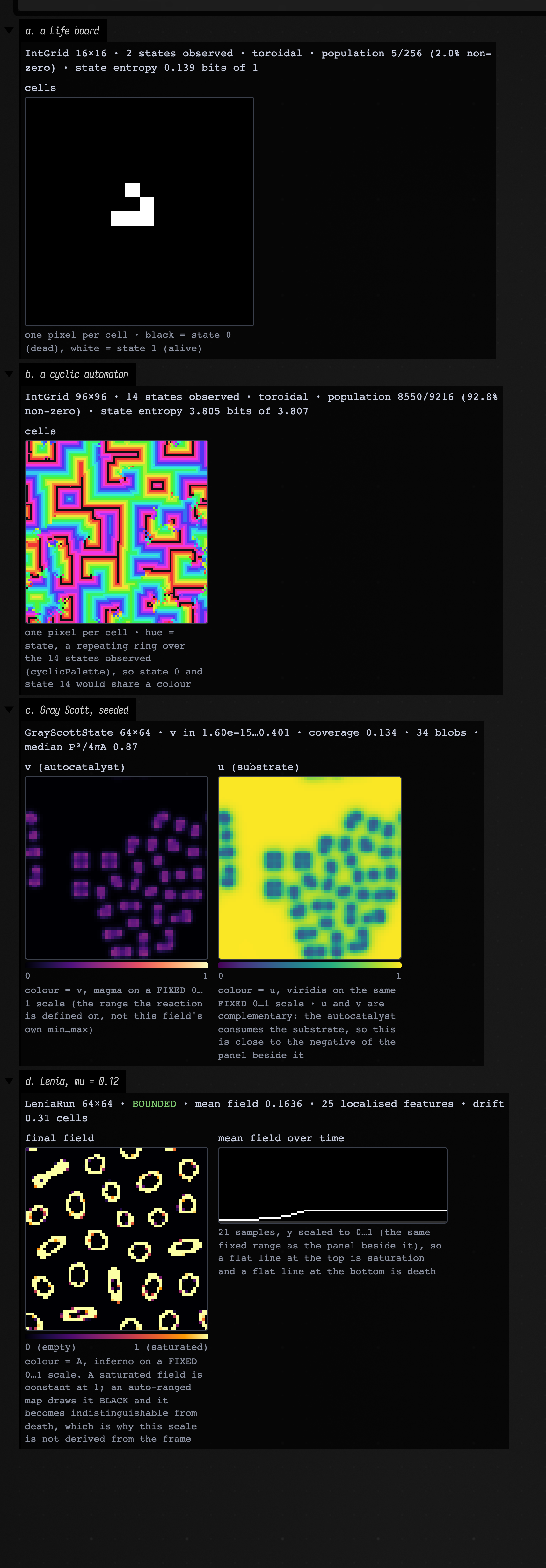

Loading all of this into a live Field

Every box above is one box of a shipped starting point, so you can open the page as a document and edit it rather than retyping it: open it from the welcome screen. Sections 1 to 10 are alife_worked_example, and section 11 is alife_evolution, kept separate because its four search boxes take about fifty seconds between them. Every box runs on its own and prints the numbers this page quotes; none of them opens a Window or a Renderer. To replay them from a terminal instead:

python3 tools/field_backdoor.py run-transcript dev_docs/agents/transcripts/alife_worked_example.yaml
python3 tools/field_backdoor.py run-transcript dev_docs/agents/transcripts/alife_evolution.yaml

The public declarations used on this page are listed, with their KDoc, in the codebase reference: alife.kt, alife_ca.kt, alife_continuous.kt, alife_agents.kt, alife_lsystem.kt and alife_field.kt. Start from what's already in the box.