Computer vision in Python

fieldcv is a small library of webcam, movie and image-sequence computer vision for Python boxes, built on OpenCV and Google's mediapipe. It finds point tracks, optical flow, moving foregrounds, body pose, hands and faces, and hands each result to the rest of Field as numpy arrays. Kotlin boxes can read those arrays, and draw them with the GPU, straight out of the same memory.

The quickest way in is the starting point. Open Starting points on the welcome screen, search for fieldcv webcam, and run its boxes from the top: your camera, mirrored, with tracks, pose, hands and a face mesh drawn over it, and a pinch of thumb and index finger that draws in the air. Browse the starting point ↗

Everything on this page runs on short clips from three public-domain films, which ship with the library so that every example works without a camera: Fernand Léger and Dudley Murphy's Ballet Mécanique (1924), the Edison company's hand-tinted Annabelle Serpentine Dance (1895), and a plate from Eadweard Muybridge's Animal Locomotion (1887). Credits are at the end.

A first look

A Pipeline takes a source of frames and any number of detectors. show() draws what every detector found into the box's output, and start() runs the pipeline on a thread of its own, so the cell returns at once and the box stays responsive while frames go by.

:::static
import fieldcv as cv4

p = cv4.Pipeline(cv4.sample("swing"), cv4.Pose(), cv4.Hands(), cv4.Face()).show().start()

The source can be a camera, a movie, or a folder of images:

cv4.Camera(0, mirror=True)               # a webcam, flipped like a selfie view
cv4.Video("dance.mp4", loop=True)        # a movie file
cv4.Images("frames/out_*.png")           # image files, in sorted order
cv4.sample("kiki")                       # one of the clips on this page

Stopping the box stops the pipeline, and running the cell again replaces it rather than starting a second one.

What a detector returns

Every detector returns a dictionary of results, including numpy arrays. Image positions are normalized: x is divided by the frame's width and y by its height, so (0, 0) is the top-left corner and (1, 1) the bottom-right. Flow vectors, listed below, are in pixels per frame. step() runs one frame on the cell's own thread, which is the easiest way to look:

:::static
import fieldcv as cv4

p = cv4.Pipeline(cv4.sample("swing", skip_seconds=4), cv4.Pose(), cv4.Hands(), cv4.Face())
r = p.step()

print(r["poses"].shape)          # (people, 33 landmarks, x y z)
print(r["hands"].shape, r["handedness"])
print(r["faces"].shape)          # (faces, 478 landmarks, x y z)
print(r["poses"][0, 0])          # the nose of the first person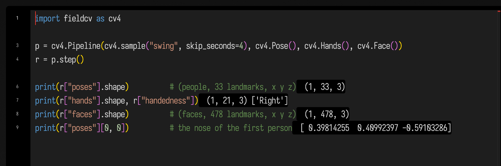

When a detector finds nothing it returns an empty array of the same shape ((0, 33, 3) for nobody in frame), never a list of NaNs, so code that loops over people simply does nothing.

The face, pose and hand models are downloaded the first time a detector needs one, into ~/.afield/models/fieldcv, and checked against a pinned hash. Pose(model="lite") is several times faster than the default and a little less steady.

Faces

Kiki de Montparnasse in the last reel of Ballet Mécanique. The face mesh holds through the superimpositions and loses her only where the frame does.

:::static
import fieldcv as cv4

p = cv4.Pipeline(cv4.sample("kiki"), cv4.Face(max_faces=3)).show().start()

Motion

Tracks follows a few hundred corners from frame to frame, and keeps a track only while it can find its way back again, so a point that slides off an edge is dropped rather than smeared. Flow measures motion at every pixel; its drawing is an arrow every sixteen pixels, and Flow.hsv(flow) is the usual full picture, hue for direction and brightness for speed.

:::static
import fieldcv as cv4

p = cv4.Pipeline(cv4.sample("machines"), cv4.Flow(), cv4.Tracks(length=12)).show().start()

Foregrounds

Background learns what the frame usually looks like and reports what is different; with contours=True it also traces the outline of each region, as normalized polylines. In Annabelle Whitford's Serpentine Dance the outline is the skirt, and pose runs alongside it on the same frames.

:::static
import fieldcv as cv4

dance = cv4.Pipeline(cv4.sample("serpentine"), cv4.Background(contours=True, min_area=0.002), cv4.Pose())
dance.show().start()

min_area is a fraction of the whole frame, so 0.002 drops anything smaller than a fifth of a percent of it at any resolution. Background("KNN"), and the contrib subtractors "GMG", "CNT" and "GSOC", trade speed for steadiness differently from the default "MOG2".

Your own drawing

show() is a convenience. Underneath it, on_result is called with every frame's results, on the pipeline's thread, and anything numpy and OpenCV can do happens there. This one keeps a canvas that fades a little every frame and draws the dancer's skeleton onto it, so Muybridge's plate becomes something like the chronophotographs it was made beside:

:::static
import cv2, numpy as np
import fieldcv as cv4
from fieldcv import field

pose = cv4.Pose()
preview = field.Preview("trails", width=640)
trails = None

def draw(r):
    global trails
    if trails is None:
        trails = np.zeros_like(r["frame"].image)
    trails[...] = trails * 0.9                                   # fade what is already there
    size = (r["width"], r["height"])
    for a, b in cv4.edges(r["poses"], pose.connections):         # one two-point line per bone
        a, b = (a * size).astype(int), (b * size).astype(int)
        cv2.line(trails, tuple(a), tuple(b), (200, 80, 255), 2, cv2.LINE_AA)
    preview.show(np.hstack([r["frame"].image, trails]))

p = cv4.Pipeline(cv4.sample("muybridge"), pose, on_result=draw).start()

field.Preview remembers the box it was made in, which is what lets it draw from the pipeline's thread.

Keeping an eye on it

A running pipeline is an ordinary Python object: run a cell that looks at it whenever you want to know how it is doing. p.latest is the newest result, p.fps the frames processed per second, and timings how long each detector took on the last frame.

:::static
import time
import fieldcv as cv4

p = cv4.Pipeline(cv4.sample("swing"), cv4.Tracks(), cv4.Pose(model="lite"), cv4.Hands()).start()
time.sleep(2)

print(p)
print({name: f"{ms:.1f} ms" for name, ms in p.latest["timings"].items()})
print(len(p.latest["tracks"]), "tracks,", len(p.latest["poses"]), "people")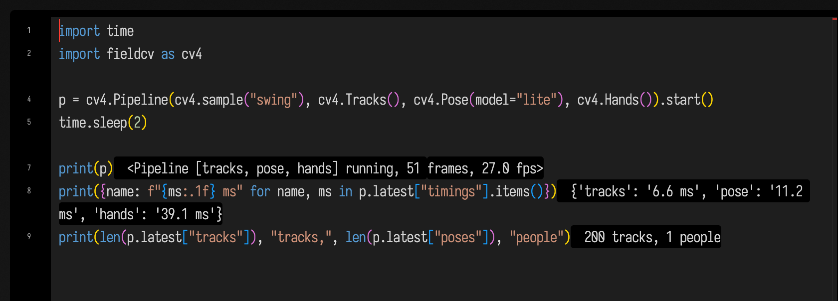

The detectors list can be changed while it runs, with p.detectors = [cv4.Hands()], and p.stop() ends it from another cell.

Into the graphics

A preview in a box's output is a JPEG sent to the browser: good for seeing what the detectors find, and no way to drive a renderer. For that, fieldcv.field puts frames and polylines in memory that a Kotlin box reads directly. field.image(name, height, width) is a (height, width, 4) numpy array whose bytes are a JVM buffer, and field.lines(name) publishes a list of polylines; on the Kotlin side NumpyShared.image(name) and NumpyShared.lines(name) find them by name.

The Python box publishes every frame from the pipeline's thread:

import fieldcv as cv4
from fieldcv import field

pose = cv4.Pose(model="lite")
camera = field.image("camera", 240, 360)
tracks = field.lines("tracks")
skeleton = field.lines("skeleton")

def publish(r):
    camera.write(r["frame"].image)          # BGR into the shared memory, then publish
    tracks.publish(r["tracks"])
    skeleton.publish(cv4.edges(r["poses"], pose.connections))

p = cv4.Pipeline(cv4.sample("swing"), cv4.Tracks(), pose, on_result=publish).start()

cv4.edges turns landmarks into one two-point line per bone, which is the shape a skeleton is drawn in. A Kotlin box under the renderer turns the shared image into a texture, which uploads only when Python has published a new frame, and puts it on a quad that fills the window:

:::static
prop<LoadedTexture>(camera) = NumpyShared.image("camera").texture()

renderer += moduleHere {
    +Mesh("camera quad") {
        // the image fills the window. Field's NDC is y-up, image v is y-down: v = 0 is the top edge
        set(4, 6) {
            pos.add(-1, -1, 0.9, 1, -1, 0.9, 1, 1, 0.9, -1, 1, 0.9)
            tc.add(0, 1, 1, 1, 1, 0, 0, 0)
            tri.add(0, 1, 2, 0, 2, 3)
        }
    }
}

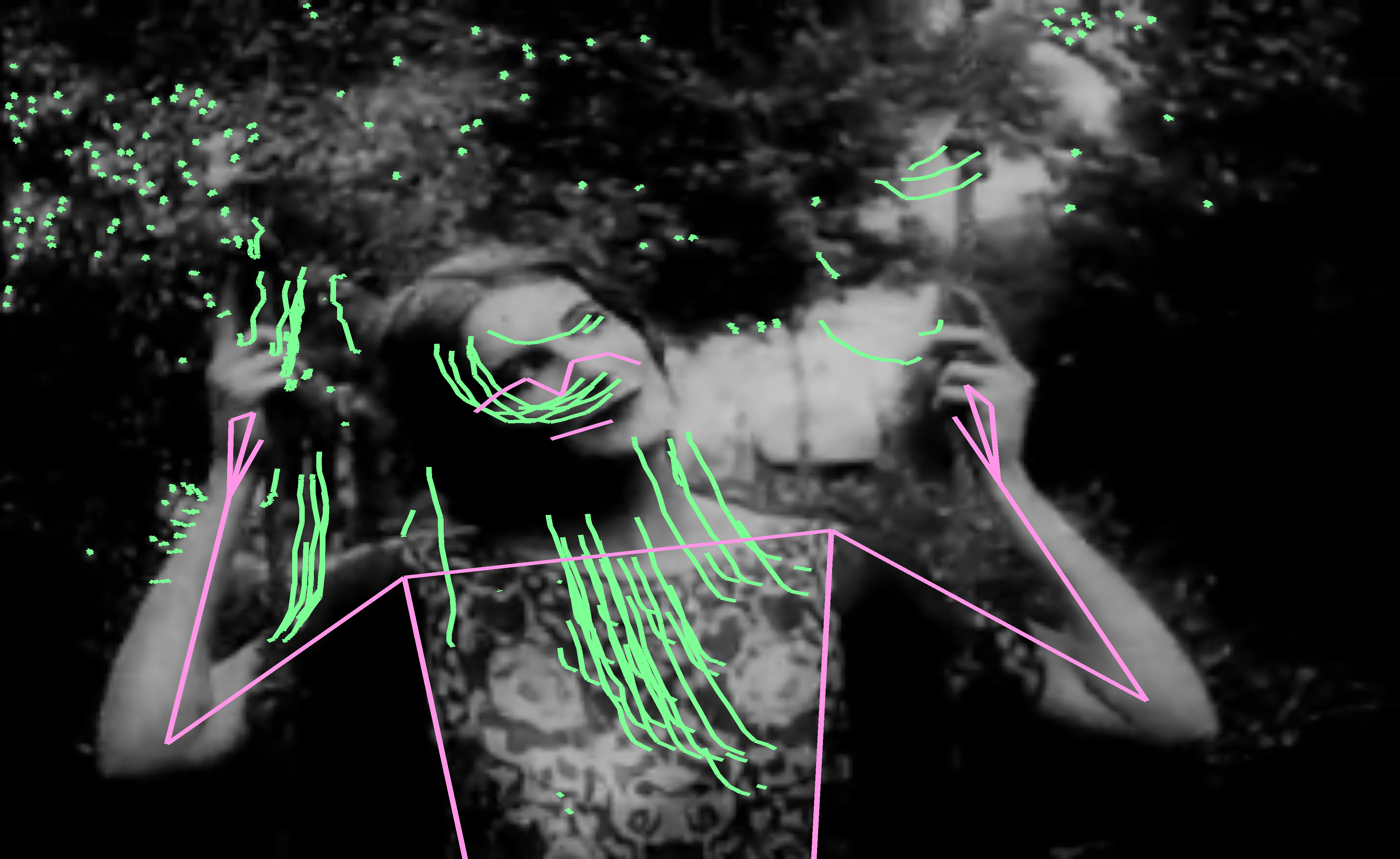
A second box draws the tracks and the skeleton, rebuilt every frame from NumpyShared.lines(...).lines(), which returns ordinary FLines. Each segment becomes a thin quad of two triangles, because a GPU line is one pixel wide whatever the window:

val tracks = NumpyShared.lines("tracks")
val skeleton = NumpyShared.lines("skeleton")

val module = moduleHere { +Mesh("overlay") }
val m = module.current.meshes.getValue("overlay")
renderer += module

val width = 0.004 // half the line's width, in NDC: about four pixels across a 1000-pixel window

fun segments(l: List<FLine>) = l.flatMap { it.nodes.zipWithNext() }

frames {
    while (frame()) {
        val segs =
            segments(tracks.lines()).map { it to vec(0.2, 1.0, 0.3, 1.0) } +
                segments(skeleton.lines()).map { it to vec(1.0, 0.3, 0.8, 1.0) }
        if (segs.isEmpty()) {
            // Publish an empty draw when detections disappear; retain no old overlay.
            m.resize(0, 0)
            continue
        }
        // each segment is a thin quad, two triangles, since GPU lines are a single pixel wide
        m.set(4 * segs.size, 2 * segs.size) {
            for ((i, s) in segs.withIndex()) {
                val (ab, c) = s
                // image (u, v), v down, to Field's y-up NDC (2u - 1, 1 - 2v)
                val ax = 2 * ab.first.to.x - 1
                val ay = 1 - 2 * ab.first.to.y
                val bx = 2 * ab.second.to.x - 1
                val by = 1 - 2 * ab.second.to.y
                val len = maxOf(Math.hypot((bx - ax).toDouble(), (by - ay).toDouble()), 1e-6)
                val nx = -(by - ay) / len * width
                val ny = (bx - ax) / len * width
                pos.add(ax + nx, ay + ny, 0.1, ax - nx, ay - ny, 0.1, bx - nx, by - ny, 0.1, bx + nx, by + ny, 0.1)
                4 { col.add(c.x, c.y, c.z, c.w) }
                tri.add(4 * i, 4 * i + 1, 4 * i + 2, 4 * i, 4 * i + 2, 4 * i + 3)
            }
        }
    }
}

One detail in both boxes is easy to get backwards: Field's normalized device coordinates have y pointing up, while an image's rows run down, so an image point (u, v) lands at (2u - 1, 1 - 2v).

The whole scene, the Python box and both Kotlin boxes, is python/fieldcv/examples/shared_memory.yaml.

Your webcam

The starting point puts all of this together on a live camera: six detectors built once and switched with use("hands", "face") while the pipeline runs, an inset in the corner showing any function of the frame you assign to inset_view (edges, the flow field, the background mask, or a one-line lambda of your own), six channels of lines drawn by one Kotlin box, and the pinch-to-draw strokes. Its second box is a list of single lines to try, one at a time.

The first time Field opens the camera, macOS asks whether the application that launched Field may use it. If Field was started from a terminal inside another application, it is that application that needs permission; the webcam box says so, and runs on a sample clip until it has it.

Installing

fieldcv lives in python/fieldcv in the Field checkout, which Field puts on Python's path at startup. Its libraries are an optional dependency group; install them into the virtual environment Field's Python uses (the one chosen in the welcome screen's Python settings):

UV_PROJECT_ENVIRONMENT=.venv uv sync --inexact --group cv --group docs --group backdoor

--inexact adds packages without removing anything already there. mediapipe is held below 1.0: the 1.0 releases end the whole process on macOS the moment a landmarker is created, and inside Field that process is Field.

Outside Field, python -m fieldcv runs the same detectors from the command line and prints one JSON object per frame, the format the old Field's contour tutorial read:

python -m fieldcv --source dance.mp4 --tracks --pose --pose-model lite > dance.jsonl

The sample clips

Each clip is a short, silent excerpt, re-encoded small, in python/fieldcv/samples.

Ballet Mécanique was published in 1924 and is in the public domain in the United States; the excerpts are taken from the copy on the Internet Archive, without its edition's title cards or its score. The Serpentine Dance (Wikimedia Commons) and the Muybridge plate (Wikimedia Commons) are in the public domain.

How the memory is shared

When a Java method hands Python a direct buffer through JEP, it arrives as a numpy array over the same bytes, and OpenCV can write into it in place: cv2.cvtColor(frame, cv2.COLOR_BGR2BGRA, dst=camera.array) is the whole of camera.write. What remains is timing: Python writes from the pipeline's thread whenever a frame is ready, and the renderer reads on its own thread at its own rate.

So each shared buffer is kept three times over. Python writes the first copy whenever it likes. publish() copies it to a second under a lock. The reader copies the second to a third, under the same lock, at the start of its frame (consume() in NumpyShared.kt), and the third copy is the only one it ever looks at, so a texture upload never shows half of one frame and half of the next. A writer that publishes faster than the renderer consumes loses frames rather than queueing them, which is what a live view wants.

Python boxes share one interpreter, so the pipeline's thread is an ordinary Python thread: it keeps running after the cell that started it returns, and it can call into the JVM. Field's Stop on its own cancels only a box's asyncio tasks, so fieldcv registers each pipeline with the box that started it and closes it when that box stops. See also Python in a Box and Field 4 graphics.