Linear programs as curves

A two-dimensional linear program asks for the point of a convex polygon that goes furthest in one direction: maximise \( c \cdot x \) over the polygon. An optimum can be found at a vertex, though an entire edge can tie. The methods here take different routes towards it. The barrier method follows a smooth arc out of the polygon's centre, the primal-dual method takes a few long strides, PDHG spirals in from outside, the ellipsoid method shrinks a sequence of ellipses around the answer, and the simplex method hops round the boundary. lpviz.net draws these routes in a browser.

In Field these routes are the product: each method returns its whole trajectory, step by step, as something you can draw, sample, animate and feed into other geometry. A polygon, an objective direction and a few dials (weights on the edges, step sizes, a centring rule) give you a family of curves that all agree about where they end.

A polygon and three routes

Build an LpPolygon from its vertices (either winding; it is normalised to counter-clockwise), pick a direction, and ask for a route. The example below draws the barrier method's central path, the primal-dual method's iterates and the simplex method's walk, all for the same direction.

:::static
val polygon = LpPolygon([vec(-2.0, -1.0), vec(1.5, -1.5), vec(3.0, 1.0), vec(0.5, 2.5), vec(-2.5, 1.5)])
val c = vec(1.0, 0.4)

val central = polygon.centralPath(c) // 160 samples as the barrier weight μ falls
val pd = polygon.primalDual(c) // one sample per Newton step
val walk = polygon.simplexWalk(c, startVertex = 4) // vertex to vertex along the boundary
:::fold draw the three panels
val outline = polygon.toFLine()
val answer = pointCloudFLine([polygon.optimalVertex(c)], vec(1.0, 0.4, 0.4, 1.0), 2.0)
val dots = { t: LpTrajectory -> pointCloudFLine(t.positions, vec(1.0, 1.0, 1.0, 0.9), 1.0) }

showPlaneGrid(
    "centralPath\n${central.samples.size} samples, μ from %.0e to %.0e"
        .format(central.samples.first().scale, central.last.scale) to [outline, central.toFLine(), answer],
    "primalDual\n${pd.samples.size - 1} Newton steps to μ = %.1e".format(pd.last.scale) to
        [outline, pd.toFLine(vec(0.55, 0.9, 0.6, 0.95)), dots(pd), answer],
    "simplexWalk\n${walk.samples.size - 1} pivots from vertex 4" to
        [outline, walk.toFLine(vec(0.6, 0.75, 1.0, 0.95), 2.4), dots(walk), answer],
    columns = 3,
    yUp = true,
    cellWidth = 310,
    cellHeight = 280,
)
:::endfold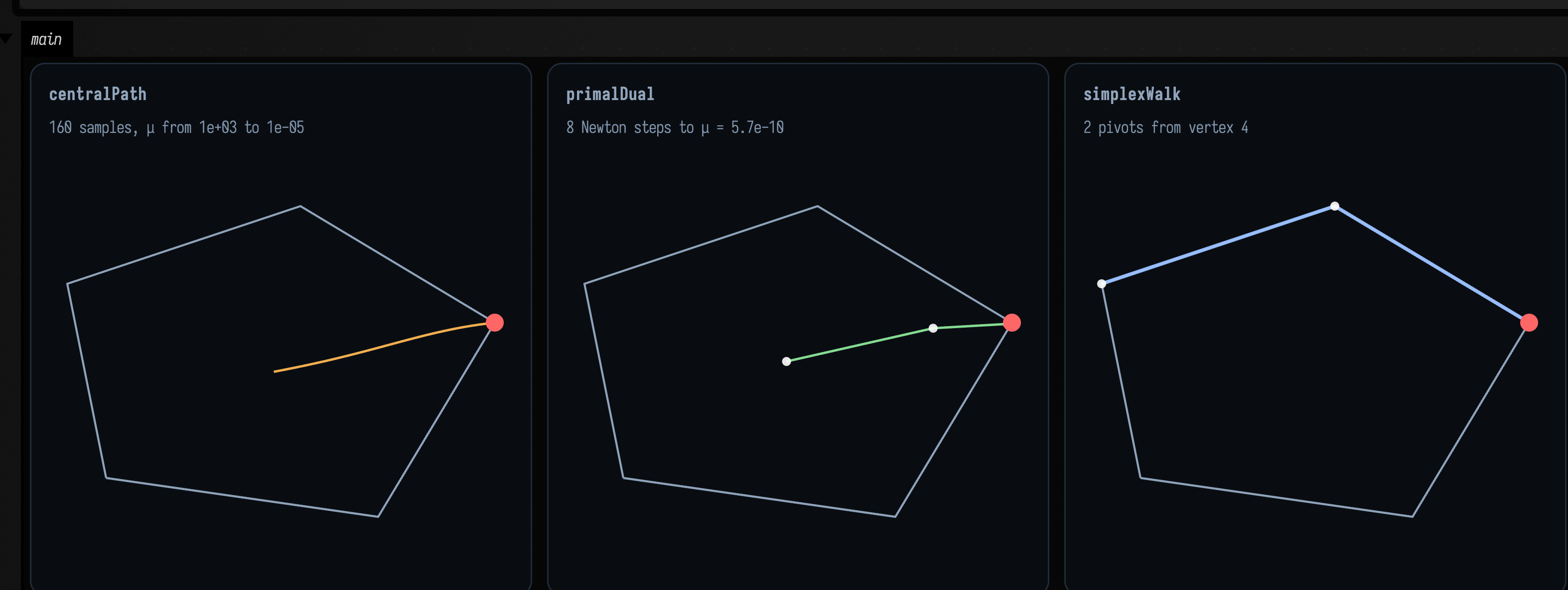

Each route is an LpTrajectory: a list of LpSamples, each carrying its position, its iteration number, its objective value \( c \cdot x \), its constraint violation, a scale and a tag. What scale measures depends on the method: μ for the two interior-point methods, the dual norm for PDHG, the ellipse's size for the ellipsoid method, the remaining area for cutting planes. toFLine() draws the route; positions gives the points.

A fan of central paths

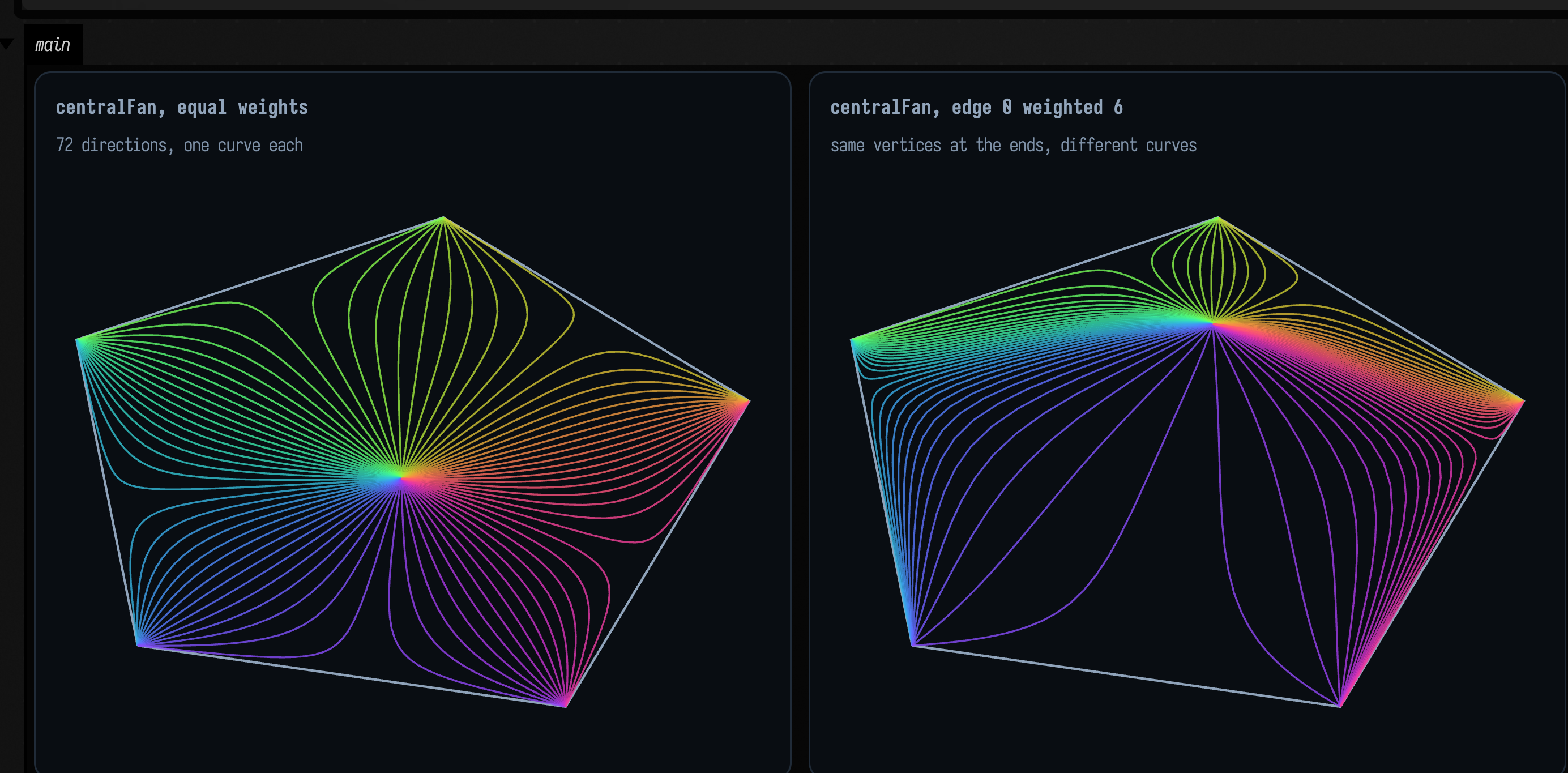
Turn the objective direction through a full circle and you get one central path per direction. All of them leave the same point (the polygon's analytic centre, where the barrier alone balances) and each ends at the vertex that wins for its direction. centralFan returns the whole family; it is a sampling of a surface \( x(\theta, \mu) \) whose two parameters are the direction's angle and the barrier weight.

:::static
val polygon = LpPolygon([vec(-2.0, -1.0), vec(1.5, -1.5), vec(3.0, 1.0), vec(0.5, 2.5), vec(-2.5, 1.5)])

val fan = polygon.centralFan(angles = 72, samples = 90)
// Weight 6 on edge 0 (the bottom-left edge) pushes every path, and the centre, away from it.
val leaning = polygon.centralFan(angles = 72, samples = 90, weights = doubleArrayOf(6.0, 1.0, 1.0, 1.0, 1.0))

showPlaneGrid(
    "centralFan, equal weights\n${fan.size} directions, one curve each" to [polygon.toFLine()] + fan.toFLines(),
    "centralFan, edge 0 weighted 6\nsame vertices at the ends, different curves" to
        [polygon.toFLine()] + leaning.toFLines(),
    columns = 2,
    yUp = true,
    cellWidth = 420,
    cellHeight = 340,
)

Weights and redundant constraints

The barrier is a sum of \( w_i \ln(\mathrm{slack}_i) \), one term per edge. Giving an edge weight 3 is exactly the same as listing that edge three times: the polygon is unchanged, but the path is not. That makes the weights a drawing control. The left panel below follows one direction with three different weightings; the right panel sweeps the weight on one edge from 1 to 40 and plots where the path starts, which is the weighted analytic centre.

:::static
val polygon = LpPolygon([vec(-2.0, -1.0), vec(1.5, -1.5), vec(3.0, 1.0), vec(0.5, 2.5), vec(-2.5, 1.5)])
val c = vec(-0.3, 1.0)

val plain = polygon.centralPath(c)
val heavyBottom = polygon.centralPath(c, weights = doubleArrayOf(8.0, 8.0, 1.0, 1.0, 1.0))
val heavyRight = polygon.centralPath(c, weights = doubleArrayOf(1.0, 1.0, 8.0, 1.0, 1.0))

// The weighted analytic centre as edge 2's weight grows: the first sample of each path.
val centres =
    (0..60).map { k ->
        val w = 1.0 + 39.0 * k / 60
        polygon.centralPath(c, weights = doubleArrayOf(1.0, 1.0, w, 1.0, 1.0), samples = 2).samples.first().position
    }
:::fold draw the two panels
showPlaneGrid(
    "three weightings, one direction\nwhite: equal, orange: edges 0 and 1 ×8, blue: edge 2 ×8" to
        [
            polygon.toFLine(),
            plain.toFLine(vec(1.0, 1.0, 1.0, 0.9)),
            heavyBottom.toFLine(vec(1.0, 0.65, 0.3, 0.95)),
            heavyRight.toFLine(vec(0.5, 0.75, 1.0, 0.95)),
        ],
    "the start moves with the weight\nedge 2 weighted 1 → 40, 61 analytic centres" to
        [
            polygon.toFLine(),
            polylineFrom(centres).also {
                it.color = vec(1.0, 0.8, 0.4, 0.9)
                it.thickness = 1.6
            },
            pointCloudFLine(centres, pointSize = 0.8),
        ],
    columns = 2,
    yUp = true,
    cellWidth = 420,
    cellHeight = 340,
)
:::endfold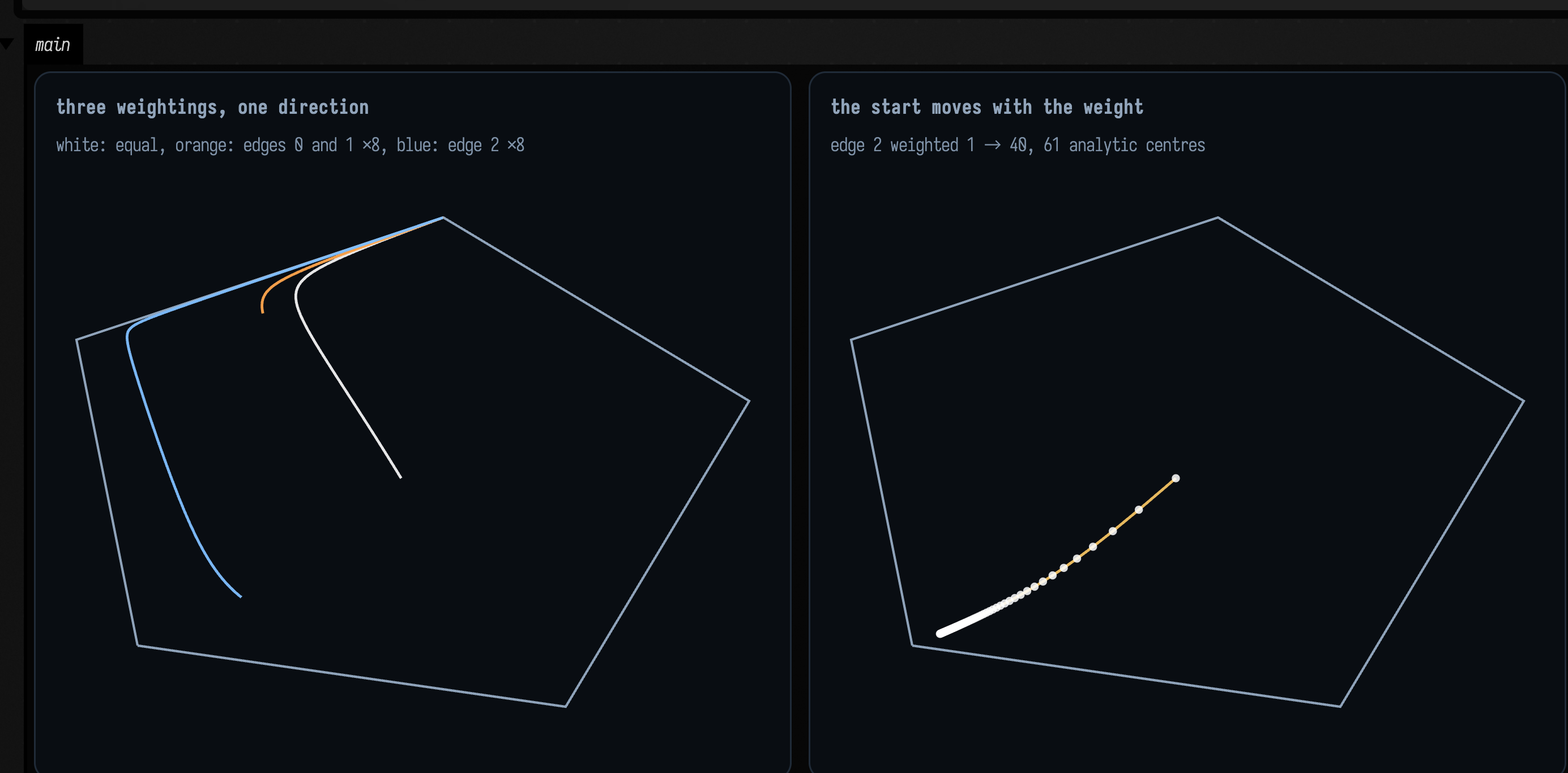

PDHG: spirals from outside

The primal-dual hybrid gradient method does no Newton solves. It keeps one dual value per edge, pushes x along the objective, and lets each edge's dual push back once x crosses it. The iterates leave the polygon, overshoot, and spiral into the vertex. pdhg keeps every state, infeasible ones included, and the duals too (trace.duals). The step sizes tau and sigma set the spiral's character: small steps wind round the vertex many times before settling, larger ones settle in a turn or two, and past the stability limit the iterates oscillate without settling, which the trace keeps.

:::static
val polygon = LpPolygon([vec(-2.0, -1.0), vec(1.5, -1.5), vec(3.0, 1.0), vec(0.5, 2.5), vec(-2.5, 1.5)])
val c = vec(1.0, 0.4)
val answer = polygon.optimalVertex(c)

val panels =
    [0.08, 0.3, 0.62].map { step ->
        val trace = polygon.pdhg(c, iterations = 700, tau = step, sigma = step)
        val end = trace.trajectory.last
        val outside = trace.trajectory.samples.count { it.violation > 0.0 }
        "tau = sigma = $step\n$outside of 701 iterates outside; ends ${end.position.distance(answer).f3} from the vertex" to
            [polygon.toFLine(), trace.trajectory.toFLine(vec(1.0, 0.55, 0.85, 0.85), 1.0)]
    }

showPlaneGrid(*panels.toTypedArray(), columns = 3, cellWidth = 310, cellHeight = 280, yUp = true)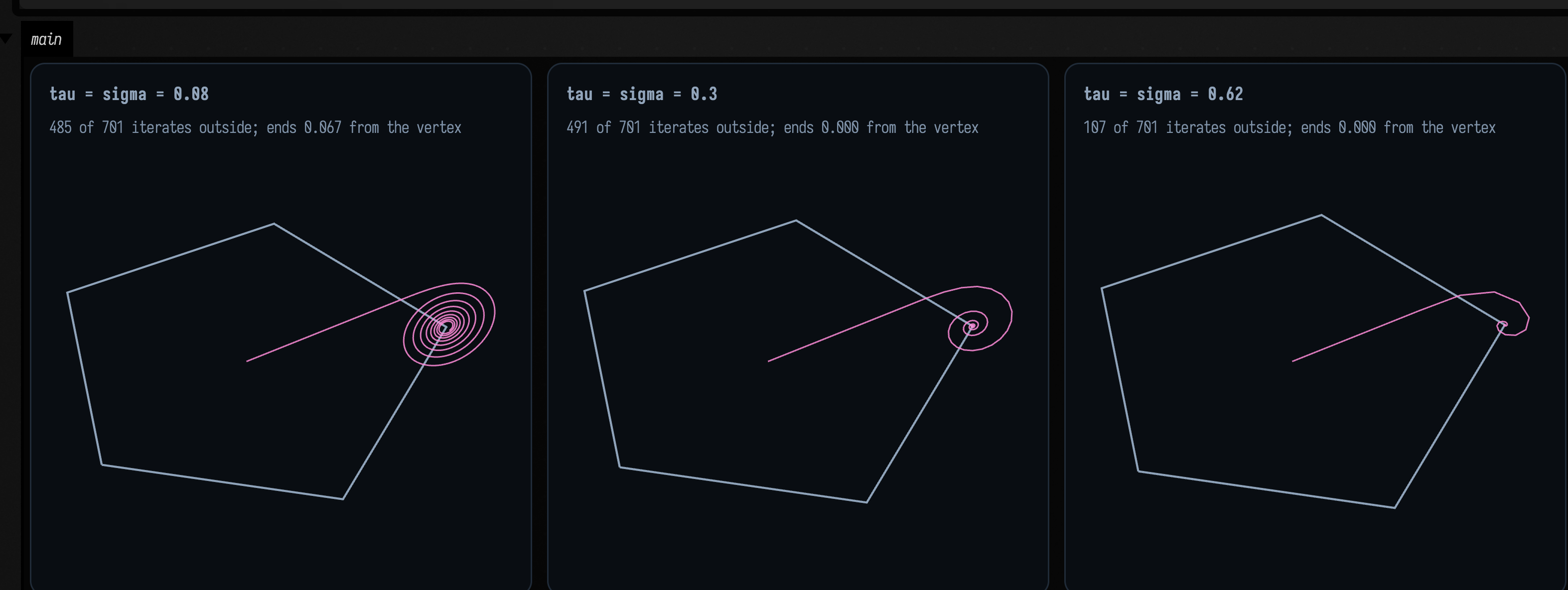

The ellipsoid method, with its ellipses

The ellipsoid method keeps an ellipse known to contain the answer. At each step it cuts the ellipse in half through its centre (on the most violated edge if the centre is outside the polygon, on the objective if it is inside) and replaces it with the smallest ellipse containing the half it keeps. In two dimensions every cut multiplies the area by \( \sqrt{16/27} \approx 0.77 \). ellipsoid returns both the centres and the ellipses (LpEllipse, a centre and a 2×2 shape matrix, with toFLine()).

:::static
val polygon = LpPolygon([vec(-2.0, -1.0), vec(1.5, -1.5), vec(3.0, 1.0), vec(0.5, 2.5), vec(-2.5, 1.5)])
val c = vec(1.0, 0.4)

val trace = polygon.ellipsoid(c, iterations = 40)
val samples = trace.trajectory.samples
val feasibilityCuts = samples.count { it.tag == "feasibility-cut" }
val best = samples.filter { it.violation == 0.0 }.maxOf { it.objective }
val optimum = polygon.simplexWalk(c).last.objective // c·x at the optimal vertex
val shrink = kotlin.math.sqrt(trace.ellipses[1].determinant / trace.ellipses[0].determinant)
:::fold draw the two panels
val ellipses = trace.ellipses.take(24).map { it.toFLine(color = vec(0.55, 0.8, 1.0, 0.35)) }
val centres = { tag: String, color: Vec4 ->
    pointCloudFLine(samples.filter { it.tag == tag }.map { it.position }, color, 1.3)
}

showPlaneGrid(
    "the first 24 ellipses\narea shrinks by ${shrink.f3} per step" to
        [polygon.toFLine()] + ellipses + trace.trajectory.toFLine(vec(1.0, 1.0, 1.0, 0.6), 0.8),
    "centres: red cut an edge, green cut the objective\n$feasibilityCuts feasibility cuts; best feasible c·x within %.1e"
        .format(optimum - best) to
        [
            polygon.toFLine(),
            trace.trajectory.toFLine(vec(1.0, 1.0, 1.0, 0.35), 0.8),
            centres("feasibility-cut", vec(1.0, 0.4, 0.4, 1.0)),
            centres("objective-cut", vec(0.4, 1.0, 0.55, 1.0)),
        ],
    columns = 2,
    yUp = true,
    cellWidth = 420,
    cellHeight = 340,
)
:::endfold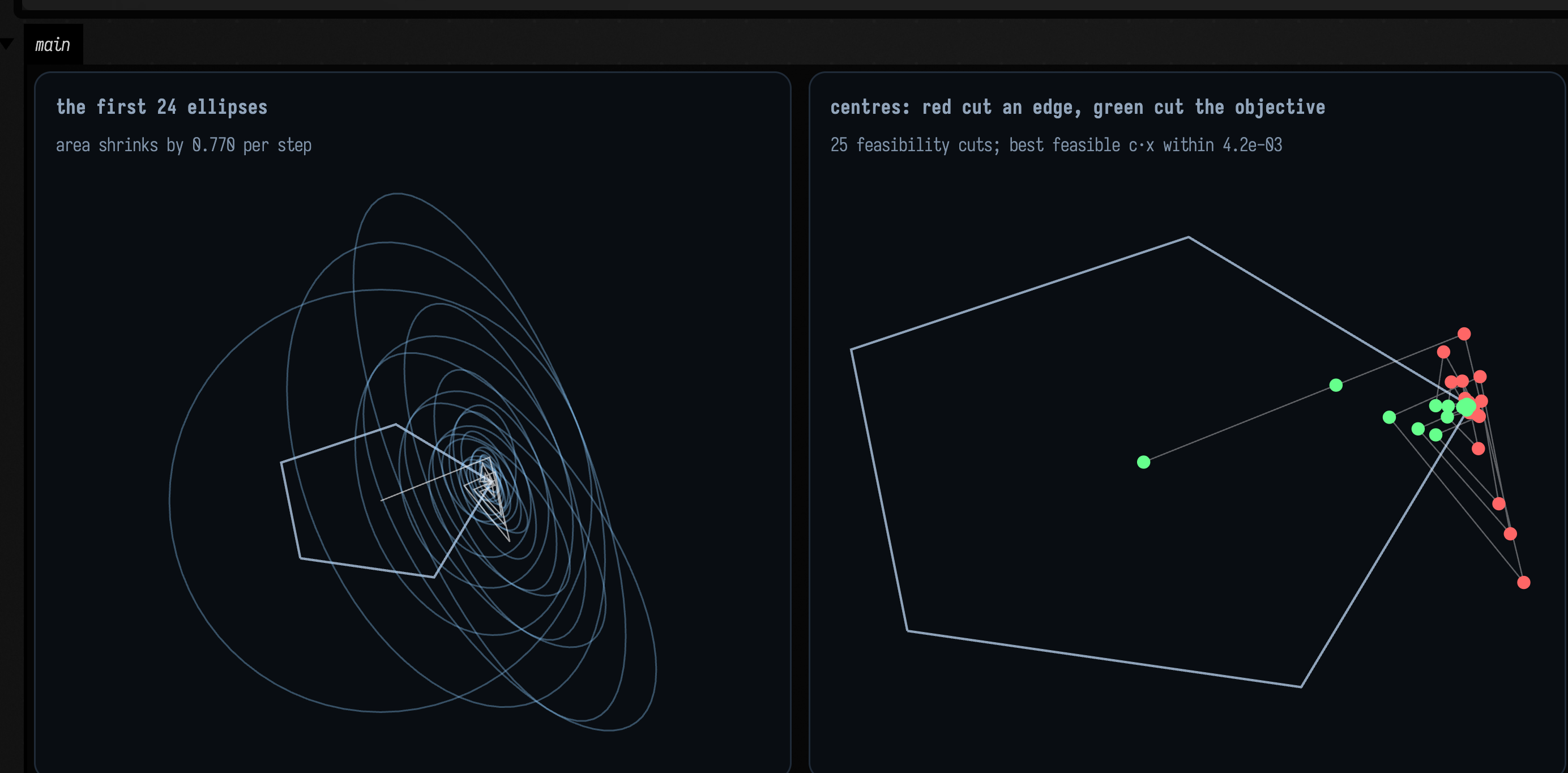

Cutting planes

A cutting-plane method keeps a region instead of an ellipse. It finds a centre of what is left, cuts away everything worse than that centre, and repeats. The four LpCenters choose the centre:

• CENTROID, the centre of gravity of the region.
• ANALYTIC, the analytic centre of every constraint so far, so each earlier cut keeps pushing, as an extra constraint pushes a central path.
• CHEBYSHEV, the centre of the largest disc that fits in the region. Only the edges the disc touches decide it.
• VOLUMETRIC, Vaidya's volumetric centre: like the analytic centre, but each constraint counts in proportion to how much it constrains, so a stack of nearly parallel cuts counts for less.

trace.regions holds the region at every step. In the example the direction (-1, -0.2) ties the two left-hand vertices, so the whole left edge is optimal and the methods may end anywhere on it: three end near its middle, while the Chebyshev centres slide down to the lower corner.

:::static
val polygon = LpPolygon([vec(-2.0, -1.0), vec(1.5, -1.5), vec(3.0, 1.0), vec(0.5, 2.5), vec(-2.5, 1.5)])
val c = vec(-1.0, -0.2)

val panels =
    LpCenter.entries.map { kind ->
        val trace = polygon.cuttingPlanes(c, iterations = 14, center = kind)
        val regions =
            trace.regions.map { r ->
                polylineFrom(r, closed = true).also {
                    it.color = vec(0.6, 0.8, 1.0, 0.4)
                    it.thickness = 0.9
                }
            }
        "$kind centres\narea %.2f → %.1e in ${trace.regions.size - 1} cuts"
            .format(trace.trajectory.samples.first().scale, trace.trajectory.last.scale) to
            [polygon.toFLine()] +
                regions +
                trace.trajectory.toFLine(vec(1.0, 0.72, 0.32, 0.95)) +
                pointCloudFLine(trace.trajectory.positions, pointSize = 1.0)
    }

showPlaneGrid(*panels.toTypedArray(), columns = 2, cellWidth = 420, cellHeight = 340, yUp = true)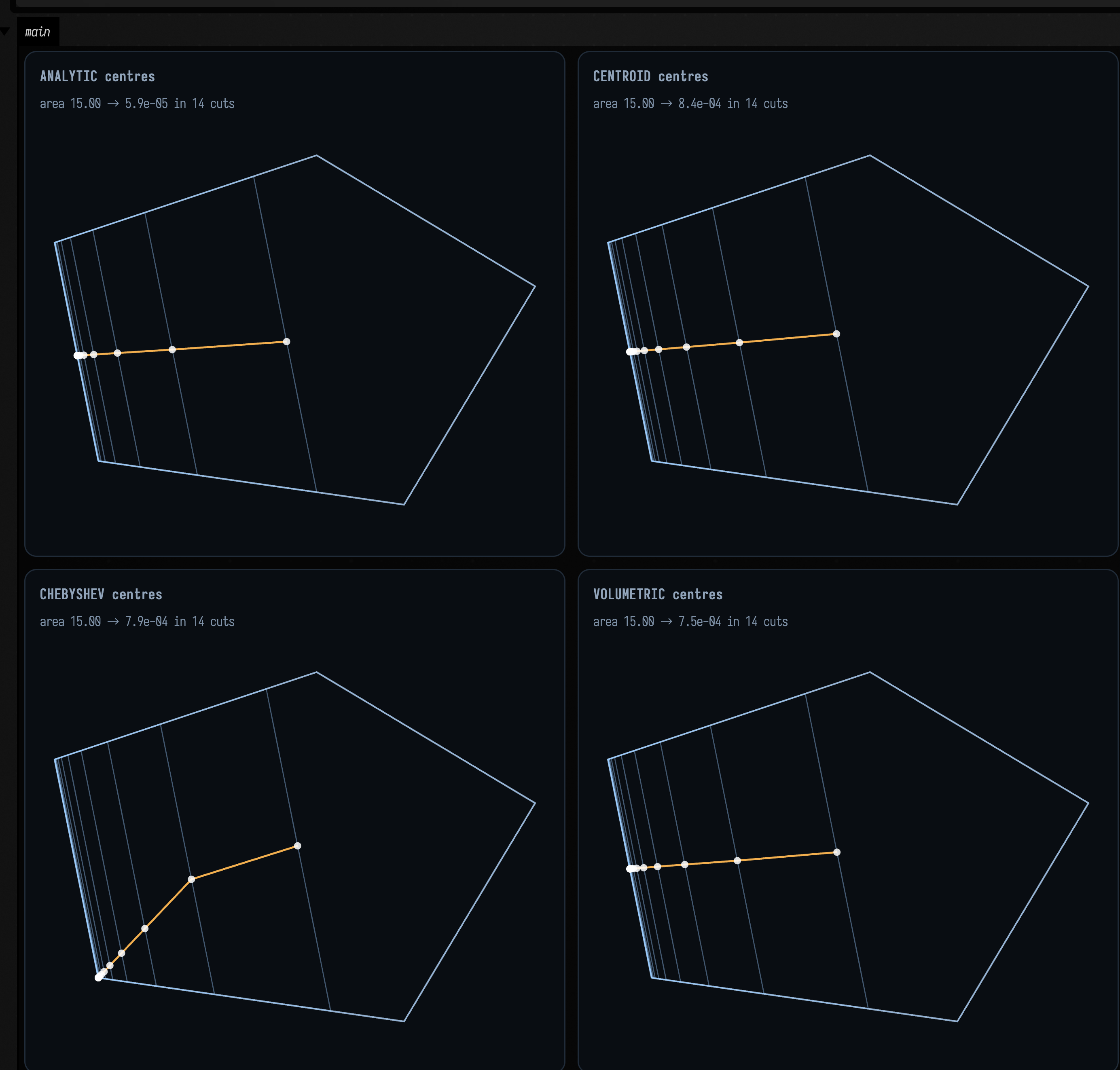

Animated: a turning objective

The objective direction below turns once every eight seconds while the hexagon's vertices breathe, and every frame redraws the central path, the PDHG spiral and the simplex walk for the new direction. The routes swing from vertex to vertex as the arrow from the centre passes each one.

The central path comes from an LpContinuation. Each frame's polygon and direction are close to the last frame's, so the continuation starts Newton for each μ at the previous frame's sample for that μ (centralPath(..., warm = previous) does the same by hand). The path is the same one a cold start would find. The caption shows both Newton step counts, and they do not always favour the warm start: when frames are close together it saves steps, but at this clip's 2.25° a frame, and while the path swings from one vertex to the next, a stale start can cost more than following the path from the centre.

:::static
val period = 8.0 // seconds per turn of the objective
val weights = doubleArrayOf(1.0, 1.0, 3.0, 1.0, 1.0, 1.0)
val window = Rect(-3.6, -3.4, 7.2, 6.8)

// Each vertex's radius wanders between 1.9 and 2.9, which keeps the hexagon convex.
fun shape(t: Double) = LpPolygon(
    (0 until 6).map { k ->
        val a = 2.0 * PI * k / 6 + 0.25
        val r = 2.4 + 0.5 * sin(t * 0.9 + k * 1.7)
        vec(r * cos(a), r * sin(a))
    },
)

val continuation = LpContinuation()
val started = AnimationClock.nowSeconds()

loop {
    val t = AnimationClock.nowSeconds() - started
    val polygon = shape(t)
    val theta = 2.0 * PI * t / period
    val c = vec(cos(theta), sin(theta))
    val central = continuation.centralPath(polygon, c, weights, samples = 90)
    val coldSteps = polygon.centralPath(c, weights, samples = 90).solverSteps
    val spiral = polygon.pdhg(c, iterations = 300, tau = 0.3, sigma = 0.3)
    val walk = polygon.simplexWalk(c)
    val o = polygon.center
    val arrow = fline {
        moveTo(o.x, o.y)
        lineTo(o.x + 0.9 * c.x, o.y + 0.9 * c.y)
        color = vec(1.0, 1.0, 1.0, 0.6)
        thickness = 1.4
    }
    showPlane(
        [
            polygon.toFLine(),
            arrow,
            spiral.trajectory.toFLine(vec(1.0, 0.55, 0.85, 0.7), 0.9),
            walk.toFLine(vec(0.6, 0.75, 1.0, 0.95), 2.4),
            central.toFLine(vec(1.0, 0.72, 0.32, 1.0), 2.0),
        ],
        title = "θ = %3.0f°".format(Math.toDegrees(theta) % 360.0),
        caption =
            "orange: central path, ${central.solverSteps} Newton steps warm, $coldSteps cold · pink: PDHG · blue: simplex walk",
        width = 560,
        height = 520,
        window = window,
        interactive = false,
        yUp = true,
    )
}

The starting point lp_curves opens the same animation in a box of its own, next to a box that draws every route at once. Change the weights or the step sizes and run it again.

Polygons from point sets and drawings

The LpPolygon constructor wants a convex polygon and says so when it is not. To run these methods over anything else (a scatter of points, a non-convex outline, a stroke drawn by hand) take its convex hull first. LpPolygon.hull(points) accepts points in any order, with repeats, and drops those inside the hull and those on a hull edge between two corners. LpPolygon.hullOf(line) does the same for the node positions of an FLine.

The example builds both: a hull of 40 scattered points, and a hull of a star whose inner corners the strict constructor would refuse as reflex. A fan of central paths runs inside each.

:::static
val random = kotlin.random.Random(5)
val points = List(40) { vec(random.nextDouble(-3.0, 3.0), random.nextDouble(-2.0, 2.0) * random.nextDouble()) }
val scattered = LpPolygon.hull(points)

// A five-pointed star: non-convex, so LpPolygon.of(star) would fail on its first inner corner.
val star = fline {
    for (k in 0..10) {
        val a = Math.PI / 2 + Math.PI * k / 5
        val r = if (k % 2 == 0) 2.6 else 1.1
        if (k == 0) moveTo(r * cos(a), r * sin(a)) else lineTo(r * cos(a), r * sin(a))
    }
    color = vec(1.0, 1.0, 1.0, 0.5)
}
val tips = LpPolygon.hullOf(star)
:::fold draw the two panels
showPlaneGrid(
    "LpPolygon.hull(points)\n${points.size} points, ${scattered.edgeCount} on the hull" to
        [scattered.toFLine()] +
            scattered.centralFan(angles = 48, samples = 80).toFLines() +
            pointCloudFLine(points, pointSize = 1.0),
    "LpPolygon.hullOf(star)\n${star.nodes.size} nodes, ${tips.edgeCount} hull vertices" to
        [star, tips.toFLine()] + tips.centralFan(angles = 48, samples = 80).toFLines(),
    columns = 2,
    yUp = true,
    cellWidth = 420,
    cellHeight = 340,
)
:::endfold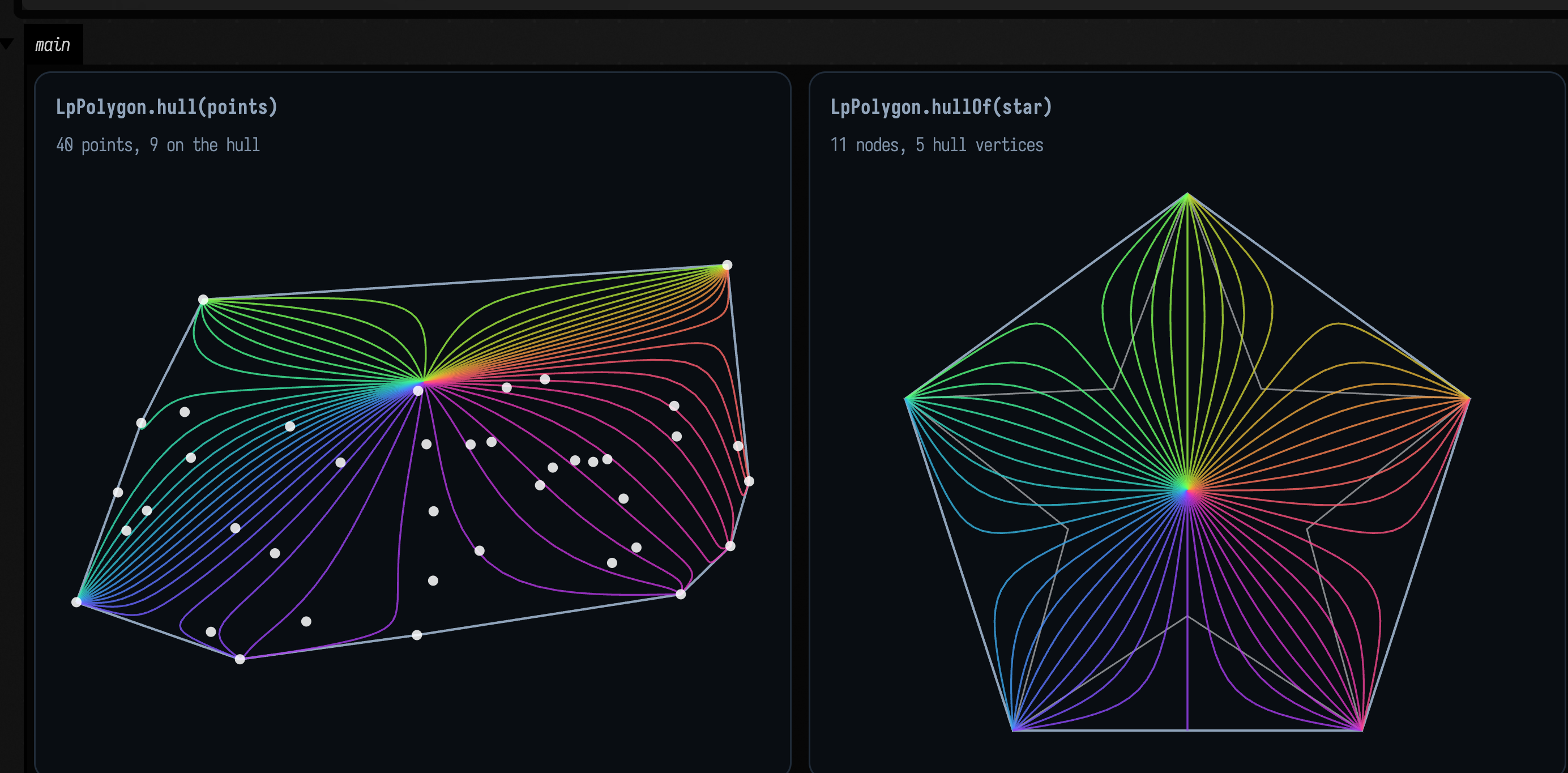

LpPolygon.of(line) and the constructor stay strict: when the outline is meant to be convex already, a reflex corner or three collinear vertices is a mistake to be told about, not something to cut off. Both read only the end point of each segment, so flatten curved segments first if their bulge should count. For a polytope in space, built the same way from a point cloud, see In three dimensions.

The fan as a map

A fan of central paths is a sampling of a map with two inputs: the objective direction's angle θ and the barrier weight μ. Give it any pair and it returns one point inside the polygon, the barrier maximiser \( x(\theta, \mu) \). polygon.fanMap() hands you that map as an object, LpFanMap. It takes \( \log \mu \) rather than μ, because the interesting range of μ spans several powers of ten.

Each point it returns, an LpFanPoint, carries the map's derivatives as well as its position: dxdTheta, how the point moves as the direction turns, and dxdLogMu, how it moves as μ grows. They are exact, not differences: at the maximiser \( c(\theta) = \mu \sum w_i n_i / s_i \), and differentiating that gives \( \partial x/\partial\theta = M^{-1} c'(\theta) \) and \( \partial x/\partial \log\mu = -M^{-1} c(\theta) \), where \( M = \mu \sum w_i n_i n_i^{\mathsf T} / s_i^2 \) is the barrier's curvature. jacobianDeterminant is the area a unit square of (θ, log μ) covers at that point, and it works out to \( 1 / \det M \), which is always positive. So the map never folds: each interior point except the analytic centre is hit by exactly one (θ, μ). In fact θ and \( 1/\mu \) are the polar angle and radius of the barrier's gradient, so the fan is polar coordinates, carried into the polygon.

fanMap().grid(thetas, logMus) samples the map on a grid and returns its coordinate lines: thetaLines() are central paths, one per angle, and muLines() are closed rings, one per value of μ. Each grid point starts Newton from an already solved neighbour, so a grid of a few thousand points takes a few milliseconds. warp(line) carries an FLine drawn in the (θ, log μ) plane, x as θ and y as \( \log \mu \), into the polygon. The example draws the grid, then a set of waves and spirals drawn in the parameter plane and warped, and then a regular lattice of dots in (θ, log μ), mapped and coloured by the determinant, in six bands of equal count from blue (smallest) to yellow (largest).

:::static
val polygon = LpPolygon([vec(-2.0, -1.0), vec(1.5, -1.5), vec(3.0, 1.0), vec(0.5, 2.5), vec(-2.5, 1.5)])
val map = polygon.fanMap()
val high = ln(100.0) // log μ at the centre end
val low = ln(1e-3) // log μ at the vertex end

val grid = map.grid(thetas = 96, logMus = 48, logMuHigh = high, logMuLow = low)

// Waves and spirals, drawn in the (θ, log μ) rectangle and carried into the polygon.
val waves =
    (0 until 9).map { k ->
        val level = high + (low - high) * (k + 0.5) / 9
        map.warp(
            fline {
                moveTo(0.0, level)
                for (s in 1..240) lineTo(2 * PI * s / 240, level + 0.35 * sin(10 * PI * s / 240))
                color = vec(0.55, 0.85, 1.0, 0.8)
            },
        )
    }
val spirals =
    (0 until 12).map { k ->
        map.warp(
            fline {
                moveTo(2 * PI * k / 12, high)
                lineTo(2 * PI * k / 12 + PI, low)
                color = vec(1.0, 0.7, 0.35, 0.8)
            },
            stepsPerSegment = 160,
        )
    }

// A lattice of dots in (θ, log μ), mapped; brighter where the map stretches area more.
val dots =
    (0 until 120).flatMap { i ->
        (0 until 40).map { j -> map.at(2 * PI * i / 120, high + (low - high) * (j + 0.5) / 40) }
    }
val logDet = dots.map { ln(it.jacobianDeterminant) }
val lo = logDet.min()
val hi = logDet.max()
:::fold draw the three panels
// Six bands by rank, so each colour holds a sixth of the dots.
val rank = logDet.indices.sortedBy { logDet[it] }.withIndex().associate { (r, k) -> k to r }
val shades =
    (0 until 6).map { b ->
        val picked = dots.filterIndexed { k, _ -> rank.getValue(k) * 6 / dots.size == b }
        val t = b / 5.0
        pointCloudFLine(
            picked.map { it.position },
            vec(0.3 + 0.7 * t, 0.35 + 0.5 * t, 1.0 - 0.6 * t, 0.9),
            pointSize = 0.5,
        )
    }

showPlaneGrid(
    "fanMap().grid(96, 48)\nθ lines are central paths, μ lines are rings" to
        [polygon.toFLine()] + grid.thetaLines(every = 3, alpha = 0.7) + grid.muLines(every = 3),
    "warp(line)\n9 waves and 12 straight lines from (θ, log μ)" to [polygon.toFLine()] + waves + spirals,
    "map.at(θ, log μ), coloured by det J\ndet from %.0e to %.0e".format(exp(lo), exp(hi)) to
        [polygon.toFLine()] + shades,
    columns = 3,
    yUp = true,
    cellWidth = 340,
    cellHeight = 300,
)
:::endfold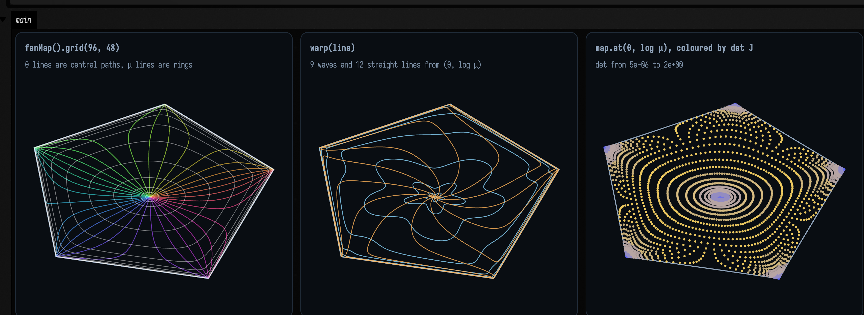

The grid shows where the map is uneven. Near the analytic centre and in the corners the cells shrink to slivers, and the determinant goes to zero: at large μ every direction lands next to the centre, as at the origin of polar coordinates, and at small μ every direction in a corner's range lands on that corner. The opposite happens along the edges. A ring of small μ crosses a whole edge within a narrow range of angles, about μ wide, so the map is steep in θ there and a grid of fixed angular step draws that crossing as one straight chord. Neither effect is a sampling error; a finer grid shows the same thing, closer to the boundary.

The same map moves particles. Below, 900 points start at random positions in (θ, log μ) and slide down in \( \log \mu \) at a steady rate, wrapping back to the top when they reach the bottom. Mapped into the polygon, each one follows its own central path out of the centre and into a corner, slowing as it goes, because the corners take up so little of the polygon. Each frame starts every point's Newton from where it was in the last frame.

:::static
val polygon = LpPolygon([vec(-2.0, -1.0), vec(1.5, -1.5), vec(3.0, 1.0), vec(0.5, 2.5), vec(-2.5, 1.5)])
val map = polygon.fanMap()
val high = ln(30.0)
val low = ln(1e-3)
val speed = 1.2 // log μ per second

val random = kotlin.random.Random(3)
val angles = List(900) { random.nextDouble(0.0, 2 * PI) }
val phases = List(900) { random.nextDouble() }
var points = angles.map { map.at(it, high) }
val paths = map.grid(thetas = 48, logMus = 40, logMuHigh = high, logMuLow = low).thetaLines(alpha = 0.25)
val started = AnimationClock.nowSeconds()

loop {
    val t = AnimationClock.nowSeconds() - started
    points = points.mapIndexed { k, p ->
        val along = (phases[k] + t * speed / (high - low)) % 1.0
        map.at(angles[k], high + (low - high) * along, near = p)
    }
    showPlane(
        [polygon.toFLine()] + paths + pointCloudFLine(points.map { it.position }, pointSize = 0.6),
        title = "900 points sliding down in log μ",
        caption = "each follows the central path for its own θ",
        width = 560,
        height = 480,
        interactive = false,
        yUp = true,
    )
}

Drag the polygon

threeLines(lines, editable = true, onEditCommitted = { edited -> … }) shows FLines in a viewer whose points you can drag with the pencil tool, and calls back with the edited lines each time a drag ends. That is enough to make the fan map editable: the first line is the polygon's outline, the callback takes the convex hull of the dragged outline (LpPolygon.hullOf, so a corner dragged inwards is dropped rather than refused) and redraws the grid for the new polygon under the same viewer name. Choose the pencil tool, then drag a corner of the white outline.

:::static
fun redraw(polygon: LpPolygon) {
    val grid = polygon.fanMap().grid(thetas = 72, logMus = 30)
    val outline = polylineFrom(polygon.vertices, closed = true).also {
        it.color = vec(1.0, 1.0, 1.0, 0.95)
        it.thickness = 2.0
    }
    threeLines(
        [outline] + grid.thetaLines(every = 2, alpha = 0.7) + grid.muLines(every = 3),
        channel = "main",
        name = "fan-map",
        height = 520,
        width = 620,
        editable = true,
        // Runs once each time a drag ends, with copies of every line as edited.
        onEditCommitted = { edited -> redraw(LpPolygon.hullOf(edited[0])) },
    )
}

redraw(LpPolygon([vec(-2.0, -1.0), vec(1.5, -1.5), vec(3.0, 1.0), vec(0.5, 2.5), vec(-2.5, 1.5)]))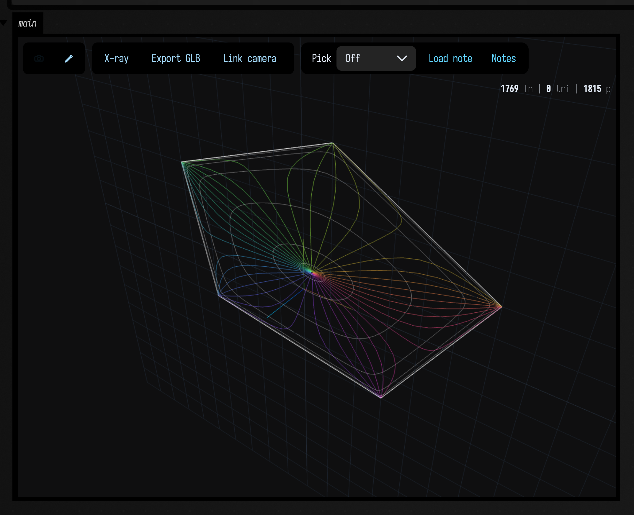

The callback runs when a drag ends, not while it moves, and the grid is recomputed then; at this size that takes a few milliseconds. The flat SVG view takes the same callback: lines(polygon, editable = true, onEditCommitted = { edited -> ... }). The starting point lp_curves has this box as lp_fan_map.

In three dimensions

Everything above works in space too. A three-dimensional linear program maximises \( c \cdot x \) over a convex polytope, the answer is again a vertex, and the same methods walk there by their own routes, now through a solid. LpPolytope holds the solid, and each method returns its walk as a 3-D trajectory that draws as an FLine in a three { } scene.

A polytope from a point cloud

LpPolytope.hull(points) takes the convex hull of any point cloud and turns each face of the hull into a half-space, the constraint \( n \cdot x \le b \). The triangles of one flat face become one constraint, so a cube has six, not twelve. LpPolytope.of(mesh) does the same for a mesh's vertices, and LpPolytope(normals, bounds) takes the half-spaces directly.

The example takes the hull of 70 points and draws a fan of central paths inside it, one per objective direction, with the directions spread evenly over the sphere. Every path leaves the polytope's analytic centre and ends at the vertex that wins for its direction.

:::static
val random = kotlin.random.Random(11)
val cloud = List(70) {
    vec(random.nextDouble(-1.6, 1.6), random.nextDouble(-1.0, 1.0), random.nextDouble(-1.0, 1.0))
}
val polytope = LpPolytope.hull(cloud)
val fan = polytope.centralFan(directions = 120, samples = 80)
:::fold draw the scene
val dots = fline {
    cloud.forEach { moveTo(it) }
    pointed = true
    stroked = false
    pointSize = 4.0
    color = vec(1.0, 1.0, 1.0, 0.7)
}
three(name = "hull-fan", width = 760, height = 470) {
    mesh(polytope.toMesh(), wireframe = false, opacity = 0.12, cullBackFaces = false)
    lines(polytope.toFLine())
    lines(dots)
    lines(fan.toFLines(alpha = 0.85, thickness = 1.2))
    camera(yaw = 32.0, pitch = 24.0)
    title("${cloud.size} points, ${polytope.vertices.size} hull vertices, ${polytope.constraintCount} faces")
    caption("${fan.size} central paths, one per direction, from the analytic centre to each direction's vertex")
}
:::endfold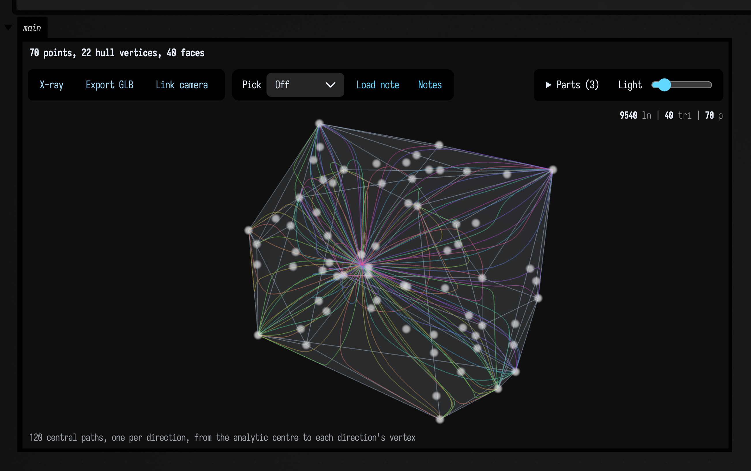

The scene can be orbited by dragging, and turntable(degreesPerSecond = …) turns it on its own. The clip below records the same scene in the Three.js viewer, with half as many paths and turntable(degreesPerSecond = 30.0). Dragging the view holds the turn, and it carries on two seconds after you let go.

:::static
val random = kotlin.random.Random(11)
val cloud = List(70) {
    vec(random.nextDouble(-1.6, 1.6), random.nextDouble(-1.0, 1.0), random.nextDouble(-1.0, 1.0))
}
val polytope = LpPolytope.hull(cloud)
val fan = polytope.centralFan(directions = 60, samples = 80)
:::fold draw the scene
val dots = fline {
    cloud.forEach { moveTo(it) }
    pointed = true
    stroked = false
    pointSize = 4.0
    color = vec(1.0, 1.0, 1.0, 0.7)
}
three(name = "turning-fan", width = 640, height = 430) {
    mesh(polytope.toMesh(), wireframe = false, opacity = 0.12, cullBackFaces = false)
    lines(polytope.toFLine())
    lines(dots)
    lines(fan.toFLines(alpha = 0.85, thickness = 1.2))
    camera(yaw = 32.0, pitch = 24.0)
    turntable(degreesPerSecond = 30.0)
    caption("${fan.size} central paths, turning")
}
:::endfold

Every route to one vertex

For a single direction, the methods take visibly different routes. The central path is a smooth arc from the centre. The primal-dual method covers the same ground in a few long strides. The simplex method walks along the polytope's edges, from vertex to neighbouring vertex, each step improving the objective. PDHG starts at the centre, overshoots the solid and spirals back in.

:::static
val random = kotlin.random.Random(11)
val cloud = List(70) {
    vec(random.nextDouble(-1.6, 1.6), random.nextDouble(-1.0, 1.0), random.nextDouble(-1.0, 1.0))
}
val polytope = LpPolytope.hull(cloud)
val c = vec(1.0, 0.5, 0.3)
val answer = polytope.optimalVertex(c)
val far = polytope.vertices.indexOf(polytope.optimalVertex(vec(-1.0, -0.5, -0.3))) // the worst vertex

val central = polytope.centralPath(c)
val pd = polytope.primalDual(c)
val walk = polytope.simplexWalk(c, startVertex = far)
val spiral = polytope.pdhg(c, iterations = 800, tau = 0.25, sigma = 0.25)
:::fold draw the scene
fun dots(t: LpTrajectory3, color: Vec4) = fline {
    t.positions.forEach { moveTo(it) }
    pointed = true
    stroked = false
    pointSize = 6.0
    this.color = color
}
three(name = "routes", width = 760, height = 470) {
    mesh(polytope.toMesh(), wireframe = false, opacity = 0.1, cullBackFaces = false)
    lines(polytope.toFLine(vec(0.62, 0.70, 0.80, 0.5)))
    lines(
        central.toFLine(vec(1.0, 0.72, 0.32, 1.0), 2.4),
        pd.toFLine(vec(0.55, 0.9, 0.6, 1.0), 1.6),
        dots(pd, vec(0.55, 0.9, 0.6, 1.0)),
        walk.toFLine(vec(0.6, 0.75, 1.0, 1.0), 3.0),
        dots(walk, vec(0.6, 0.75, 1.0, 1.0)),
        spiral.trajectory.toFLine(vec(1.0, 0.55, 0.85, 0.8), 1.0),
    )
    camera(yaw = 20.0, pitch = 20.0)
    title("c = (1, 0.5, 0.3): four routes to the vertex at (${answer.x.f2}, ${answer.y.f2}, ${answer.z.f2})")
    caption(
        "orange: central path · green: primal-dual, ${pd.samples.size - 1} steps · blue: simplex, ${walk.samples.size - 1} pivots along edges · pink: PDHG",
    )
}
:::endfold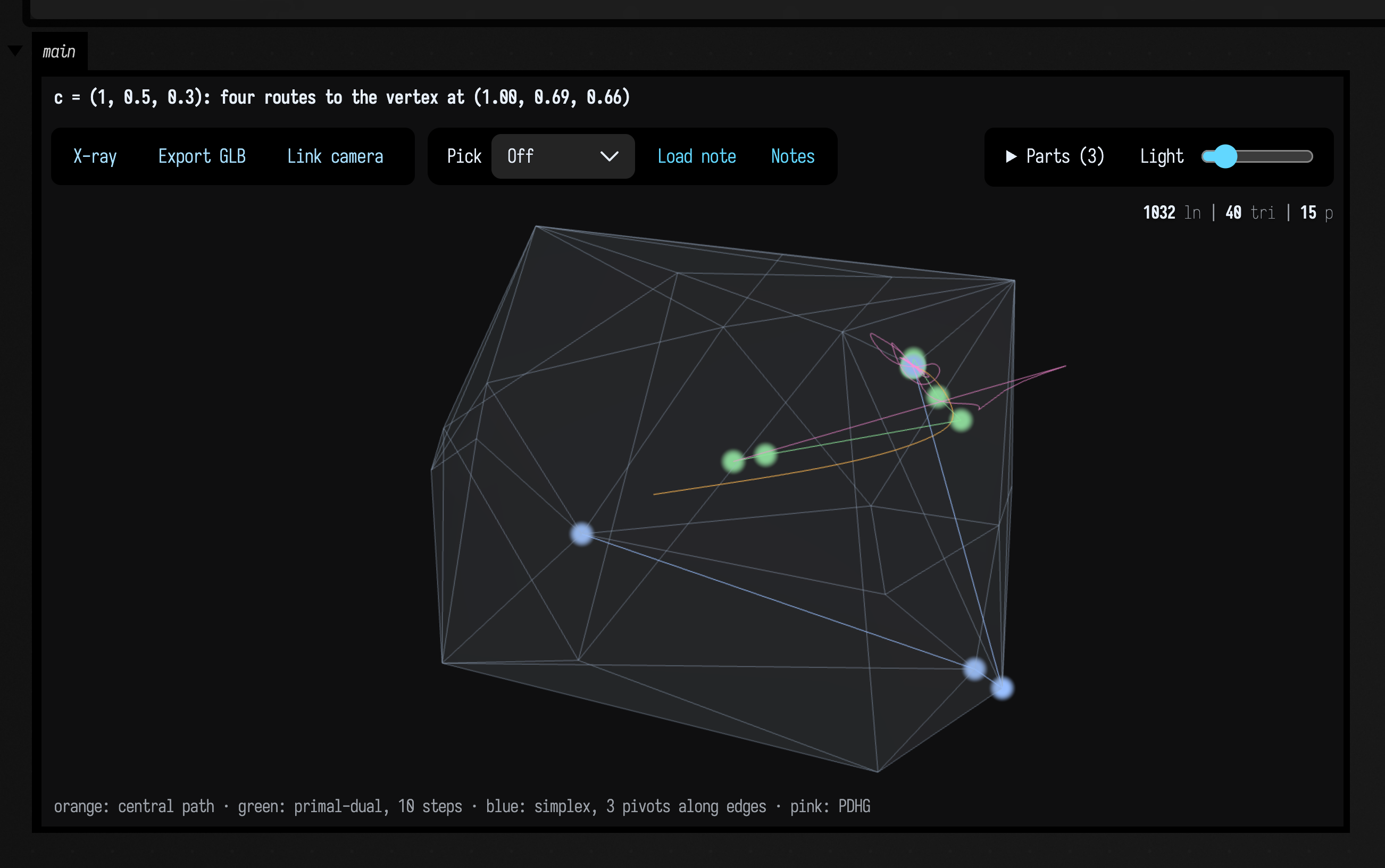

The trajectories are LpTrajectory3s of LpSample3s, carrying the same per-step data as in 2-D (position, iteration, objective, violation, scale, tag), and toFLine() draws each one as a 3-D polyline.

Ellipsoids

The ellipsoid method keeps an ellipsoid known to contain the answer, halves it through its centre at each step, and replaces it by the smallest ellipsoid containing the half it keeps. The constants depend on the dimension. In three dimensions the centre moves a quarter of the way across (1/(n+1)), the shape matrix grows by \( n^2/(n^2-1) = 9/8 \), and each step multiplies the volume by \( 27/32 \approx 0.84 \), a slower shrink than the plane's 0.77. LpEllipsoid.toFLine() draws an ellipsoid as a wireframe of latitude and longitude rings.

:::static
val cube = LpPolytope.cube(1.0)
val c = vec(1.0, 0.6, 0.3)

// Start from a ball of radius 2, just larger than the cube's circumscribed sphere (√3).
val trace = cube.ellipsoid(c, iterations = 60, initialRadius = 2.0)
val shrink = kotlin.math.sqrt(trace.ellipsoids[1].determinant / trace.ellipsoids[0].determinant)
val best = trace.trajectory.samples.filter { it.violation == 0.0 }.maxBy { it.objective }
:::fold draw the scene
three(name = "ellipsoids", width = 760, height = 470) {
    lines(cube.toFLine(vec(1.0, 1.0, 1.0, 0.8), 1.6))
    lines((0..24 step 8).map { trace.ellipsoids[it].toFLine(rings = 4, color = vec(0.55, 0.8, 1.0, 0.5)) })
    lines(trace.trajectory.toFLine(vec(1.0, 0.72, 0.32, 0.9), 1.4))
    camera(yaw = 28.0, pitch = 22.0)
    helpers(false)
    title("ellipsoids 0, 8, 16 and 24; each step keeps ${shrink.f3} of the volume")
    caption(
        "orange: the ${trace.trajectory.samples.size} centres; best feasible centre (${best.x.f3}, ${best.y.f3}, ${best.z.f3}), optimum (1, 1, 1)",
    )
}
:::endfold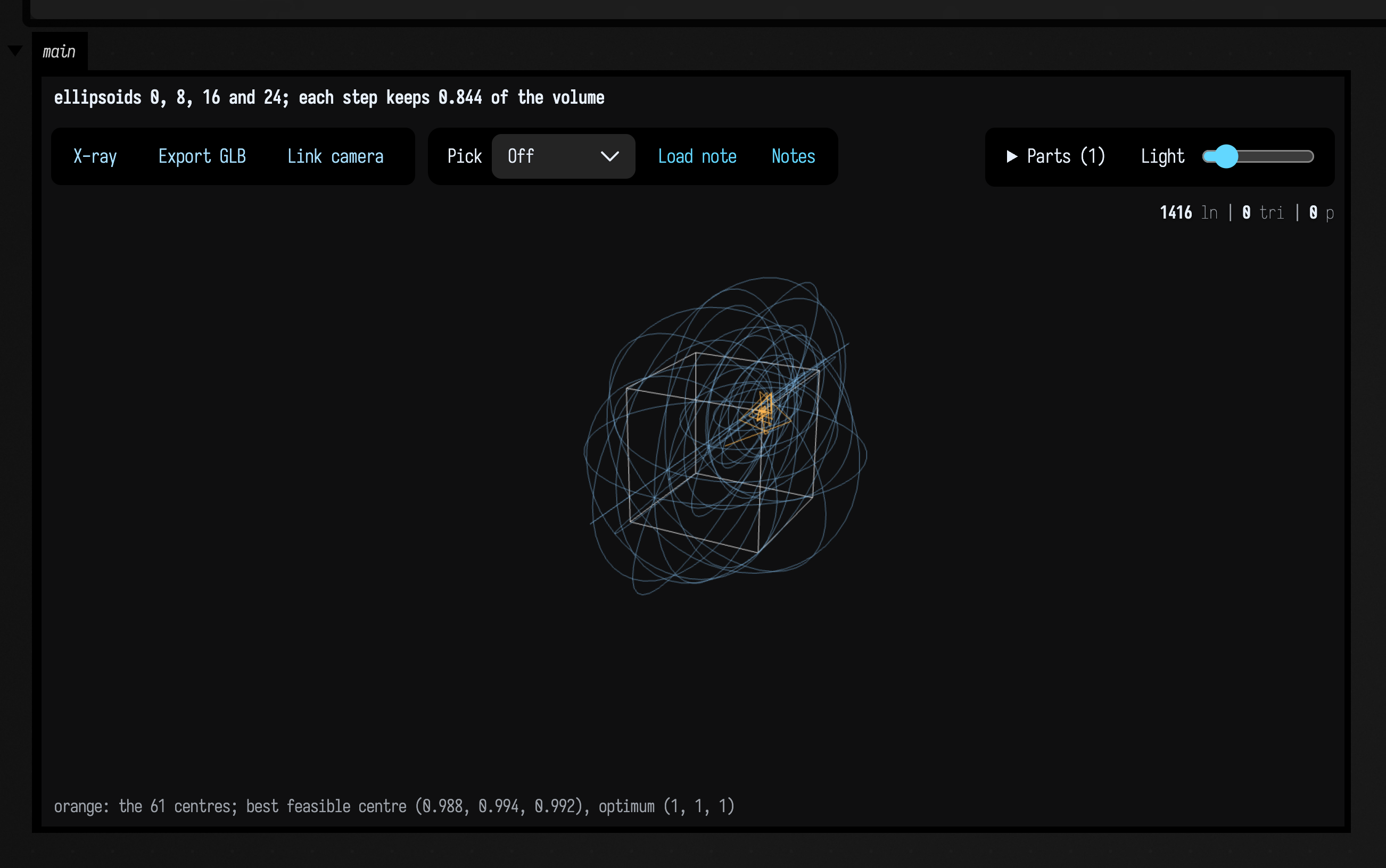

Cutting planes

A cutting-plane method keeps the region still in play, finds a centre of it, and cuts away the half where \( c \cdot x \) is worse than at the centre. cuttingPlanes returns the region at every step as an LpPolytope of its own. In three dimensions the centre is ANALYTIC, CENTROID, CHEBYSHEV (the centre of the largest ball inside) or VOLUMETRIC, as in the plane. The example cuts toward the cube's top corner through centroids, each of which removes at least \( 1 - (3/4)^3 \approx 58\% \) of the volume.

:::static
val cube = LpPolytope.cube(1.0)
val c = vec(1.0, 0.6, 0.3)

val trace = cube.cuttingPlanes(c, iterations = 8, center = LpCenter.CENTROID)
val volumes = trace.trajectory.samples.map { it.scale }
:::fold draw the scene
three(name = "cuts", width = 760, height = 470) {
    trace.regions.forEachIndexed { k, region ->
        val t = k / (trace.regions.size - 1.0)
        lines(region.toFLine(vec(0.5 + 0.5 * t, 0.8 - 0.2 * t, 1.0 - 0.6 * t, 0.35 + 0.6 * t), 1.0 + t))
    }
    lines(trace.trajectory.toFLine(vec(1.0, 1.0, 1.0, 0.9), 2.0))
    camera(yaw = 28.0, pitch = 22.0)
    helpers(false)
    title(
        "centroid cuts toward (1, 1, 1): volume ${volumes.first().f1} → ${volumes.last().f4} in ${volumes.size - 1} cuts",
    )
    caption("each region is drawn as its edges, blue first and orange last; white: the path of centroids")
}
:::endfold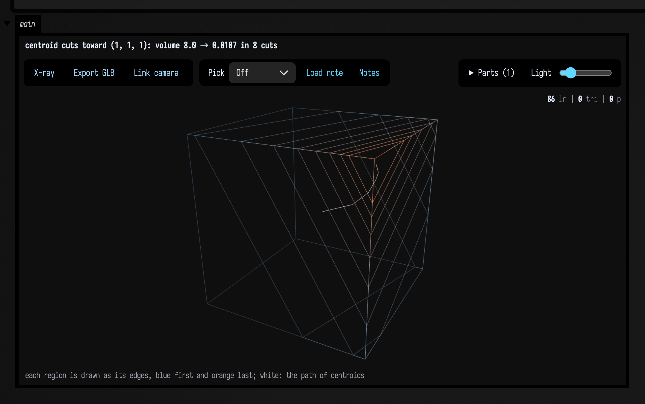

The starting point lp_curves_3d opens a hull with every route in one box and the turning fan in another.

Reference

In three dimensions:

Source: src/jvmMain/kotlin/afield/geometry/spatial/lp_trajectories.kt, src/jvmMain/kotlin/afield/geometry/spatial/lp_fan_map.kt and src/jvmMain/kotlin/afield/geometry/spatial/lp_polytope.kt.

The public declarations used on this page are listed, with their KDoc, in the codebase reference: Graphics.