Neural particle systems
Give a particle system a picture to make, and let a small neural network learn how to move the particles into place. Here it has assembled 300,000 particles into the word FIELD:
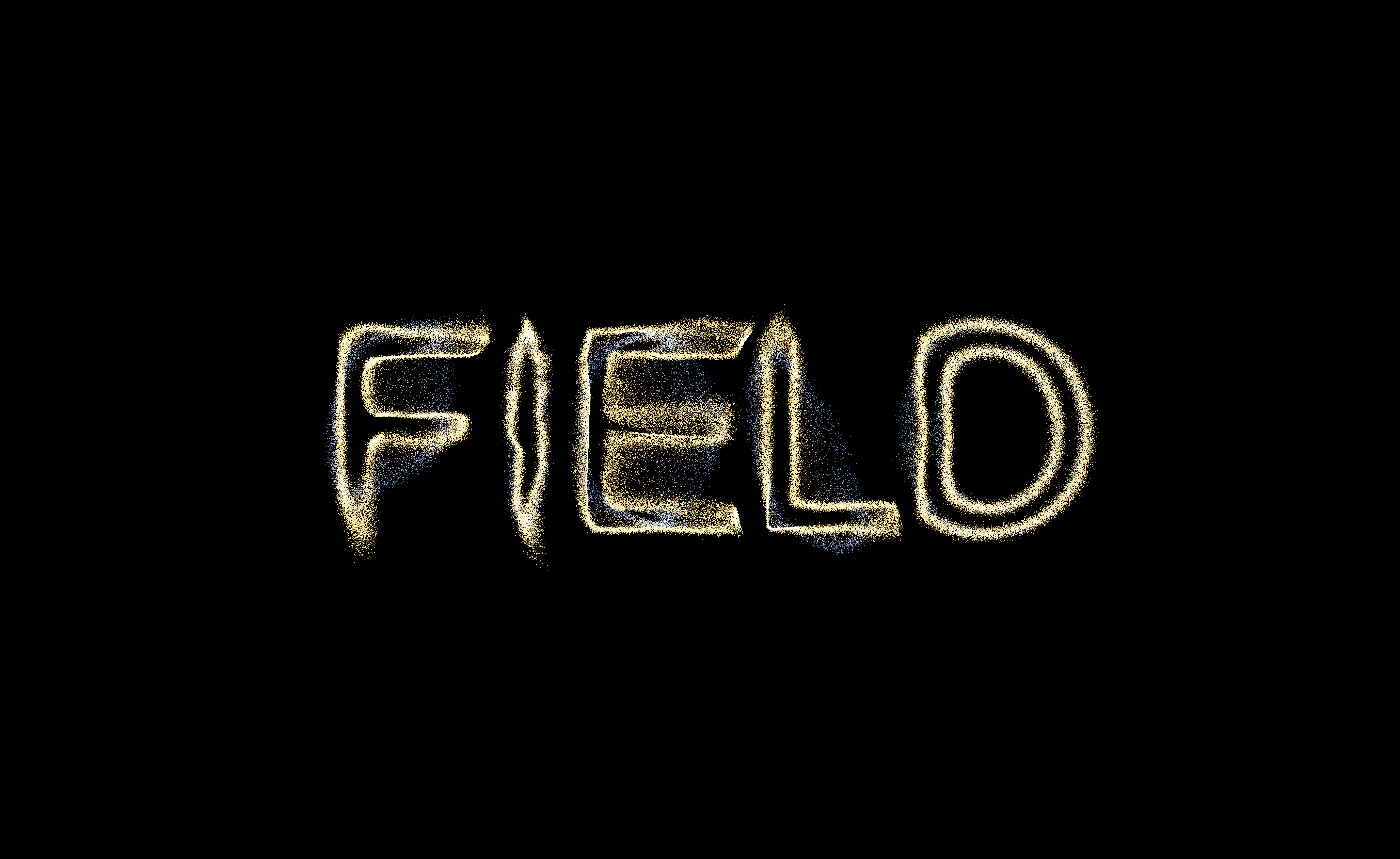
Three hundred thousand particles, each asking a small neural network where to go next, every frame. The rule that assembles them into that word was fitted in about a second of Kotlin and then compiled into a shader.
A particle system is normally something you write: a few lines of arithmetic, run over a million points. That works when you know the arithmetic. When what you have is a shape you want the cloud to become, or a behaviour you can recognise but not write down, the usual answer is tuning coefficients until the picture looks right, which is slow, hard to repeat, and gets harder with every parameter you add.
Fit the rule instead when:
- You can state the destination but not the route. "Become these letters" is easy to specify and hard to hand-write as a velocity field. Training takes a second and the answer runs live.
- You have a rule that is expensive, and want a cheap one that behaves like it. A learned rule costs the same every frame no matter how intricate the thing it imitates.
- The target changes and you do not want to re-derive anything. Retraining is a couple of seconds and swaps a buffer; the shader is never recompiled. In the first scene below the target is a string you can edit while it runs.
A trained rule that looks convincing is easy to get: almost any attraction-and-repulsion rule with a speed limit produces something an audience will accept as flocking. So the learned rules here are compared against a written rule that does the same job.
The first section covers the part in between, which you can use on its own: turning a network trained in Kotlin into a GLSL forward pass that runs once per particle.
Particle rules that were trained
There are two kinds of rule a particle can follow. The first reads only its own state: a velocity
field v(x, t), blind to every other particle in the buffer. The second reads its neighbours: a
force that depends on the particles nearby.
Field fits either one. A velocity field moves particles toward a target shape; an interaction produces forces from their neighbours, making flocks, swarms and crowds. The latter needs a neighbour search to run efficiently.
The two are built in that order below: tier one is sections 1 to 3, the neighbour search is section 4, and tier two is sections 5 to 7.
Source files
| file | what is in it |
|---|---|
afield/simulation/particles/neuralparticles.kt |
MlpWeights, MlpWeights.glsl, FlowMatchExport, blendWith, MlpAgreement — the network-to-shader bridge |
afield/simulation/particles/neuralparticles_system.kt |
ShaderNeuralParticles, NeuralParticleSettings — tier one, as a running system |
afield/ai/learning/flowmatching.kt |
flowMatch, contourComponents, mixtureSource — the CPU half, shared with Flow matching |
afield/ai/learning/deepsets.kt |
trainDeepSets, trainEquivariant, and their GLSL emitters — tier two's learned rule |
afield/graphics/vulkan/util/GpuNeighbourGrid.kt |
hash, sort, ranges: the neighbour search both flocks share |
afield/simulation/physics/ShaderBoids.kt |
ShaderBoids, BoidSettings: the written rule and the learned one, in one system |
Four transcripts open as complete documents from Agent transcripts or the
welcome screen: neural_particles, learned_boids, letter_interpolation and
letter_interpolation_panels. Everything below is reachable from one of them, and they are
the fastest way in: open one, edit a number, watch it change.
1. A trained field, running as a shader
Flow matching fits v(x, t) by least squares in about a second of pure Kotlin.
Three calls take that network to the GPU:
val field = flowMatch(pairing.to, pairing.from, FlowMatchOptions(coupling = FlowCoupling.PAIRED))
val export = field.export() // weights, training frame, source cloud
val glsl = export.glsl("neuralField") // place this immediately after #version
export() is a snapshot: the weights flat and layer-major, plus the centring and scaling the
network was trained in, plus the source cloud so the system knows where particles start.
glsl(name) emits an unrolled forward pass that reads those weights out of a storage buffer rather
than baking them in as literals, so retraining swaps a buffer between frames and never
recompiles a shader. The layer loop is unrolled and the dot products are not, so the emitted
source stays proportional to the depth of the network: a five-thousand-parameter net is still
readable GLSL.
ShaderNeuralParticles is the system that runs it:
val particles = ShaderNeuralParticles(export) {
    particleCount = 300_000
    stepsPerCycle = 150
    dwellCycles = 3f // how long a particle rests on the target once it arrives
}
particles.installInto() // defaults to renderer.renderList
Each particle is a struct rather than a texel, because of the two unusual fields:
struct Particle {
    vec2 position;
    vec2 start;
    vec2 velocity;
    float t;
    float pad;
};
A flow is a map. Each particle travels from one specific source point to wherever the field takes it by t = 1, and when it arrives it goes back
and does it again. start and t are what make that possible, and neither fits in a four-channel
texel.
One forward pass per particle per frame. The default flow-matching network is 11 -> 64 -> 64 -> 2,
about five thousand multiply-adds, so two hundred thousand particles is roughly a GFLOP a frame.
Width is a cheaper dial than count: a 32 x 32 network is four times less work, and a 2D
flow rarely needs 64.
When the picture is a haze
If the picture is a haze, reach for dwellCycles first. A particle that resets the instant it
reaches t = 1 is on the target for exactly one frame out of stepsPerCycle, so with phases
spread out only a hundred and fiftieth of the cloud is ever on the shape, and the rest, still in
transit, drown it. At 0f a correctly trained
300,000-particle system renders a featureless smudge that looks exactly like an undertrained field.
At the default of 3f a particle spends three quarters of its life arrived.
Set it to 0f to see the flow alone, or very high to see only the distribution.
2. Making your own target
The image at the top of this page is the word FIELD. Getting a word rather than a single letter needs one piece of work that has nothing to do with the GPU, and it is the piece you will need for any target that comes in more than one part.
Integrating a velocity field is a continuous invertible map. It can deform a blob but it cannot
tear one into five, so a standard Gaussian source cannot become the five disjoint outlines of a
word, however long you train and however big the network. mixtureSource fixes it by giving
the source the target's topology: one ellipse per closed subpath, fitted to that subpath's own
mean and covariance, in point-for-point correspondence with the contour it has to become.
val contours = layoutText("FIELD", typeface("Helvetica", 260.0)).toFLines()
val pairing = mixtureSource(contourComponents(contours, total = 12000), seed = 5)
val field = flowMatch(pairing.to, pairing.from, FlowMatchOptions(coupling = FlowCoupling.PAIRED))
contourComponents splits the outlines into closed subpaths and samples each in proportion to its
length; mixtureSource fits an ellipse to each and pairs it, point for point, with its contour.
FlowCoupling.PAIRED is what tells flowMatch to respect that pairing instead of drawing its own.
Here is that construction on its own, on the CPU: the source it builds, drawn against the target it has to reach.
:::static
val contours = layoutText("Fi", typeface("Helvetica", 300.0)).toFLines()
val components = contourComponents(contours, total = 2400, seed = 7)
val pairing = mixtureSource(components, seed = 5)

fun cloud(points: List<Vec3>, size: Double, c: Vec4): FLine {
    val f = FLine()
    points.forEach { f.moveTo(it) }
    f.pointed = true
    f.pointSize = size
    f.color = c
    return f
}

// Every 100th correspondence, to show the pairing is point-for-point and not a cloud match.
val threads = FLine()
for (i in pairing.from.indices step 100) {
    threads.moveTo(pairing.from[i])
    threads.lineTo(pairing.to[i])
}
threads.color = vec(1.0, 0.62, 0.25, 0.75)
threads.thickness = 1.2
:::fold draw the source, the target and the pairing
lines(
    [
        cloud(pairing.to, 2.0, vec(0.55, 0.55, 0.62, 0.9)),
        cloud(pairing.from, 1.6, vec(0.44, 0.83, 0.78, 1.0)),
        threads,
    ],
    w = 1000.0,
    h = 450.0,
    fitToSize = true,
)
markdown(
    "what",
    """
    ~~~
closed subpaths found   ${components.size}
points per component    ${components.map { it.size }.joinToString(", ")}
paired points           ${pairing.from.size}
    ~~~
""",
)
:::endfold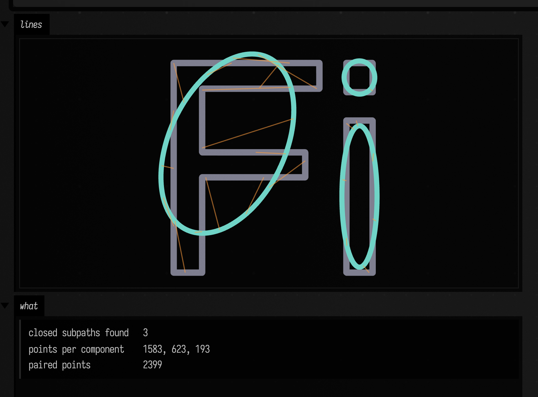
Grey is the target, the letter outlines. Teal is the source the flow starts from: one ellipse per closed subpath, so the "i" arrives as two components, its stem and its dot, each with its own ellipse. A letter with a counter (a "D", an "e") would contribute two as well, outer and inner. Orange threads are the correspondence, every hundredth pair. The flow's whole job is to shorten those threads.
Three choices inside that construction have defaults you should keep:
| what | if you turn it off | why |
|---|---|---|
| subpaths, not glyphs | contourComponents given whole letters |
a "D" becomes one annulus, and its counter has to be torn open |
alignPhase = true |
identity pairing | a contour's arc-length origin has nothing to do with angle zero on its ellipse, so every component carries an arbitrary rotation the flow must unwind |
| no jitter on the source | jitter above zero |
the ellipse thickens to an annulus and the correspondence blurs |
alignPhase is the least obvious of the three and changes the result most. To see it, open the
neural_particles scene, set it to false, retrain, and watch the letters arrive twisted.
Almost every setting in that scene is live, including the text. Retraining takes a couple of seconds.
3. Between two trained fields
Train a second field, from the same source, and you can interpolate the weights:
val blended = fieldA.blendWith(fieldB, t) // t from 0 to 1
particles.updateWeights(blended.network) // a buffer write; nothing recompiles
Interpolating the targets, sending point i to \( (1-t)\,A_i + t\,B_i \), is a straight-line
crossfade that needs no network. Interpolating the weights gives a field that was never trained
on anything, and where it sends a particle is a nonlinear function of t.
The two give very different results. Measured at t = 0.5, the weight-space landing sits 0.85 of the
whole width of the morph from where the crossfade would put it — nearly as far as the two
letters are from each other.
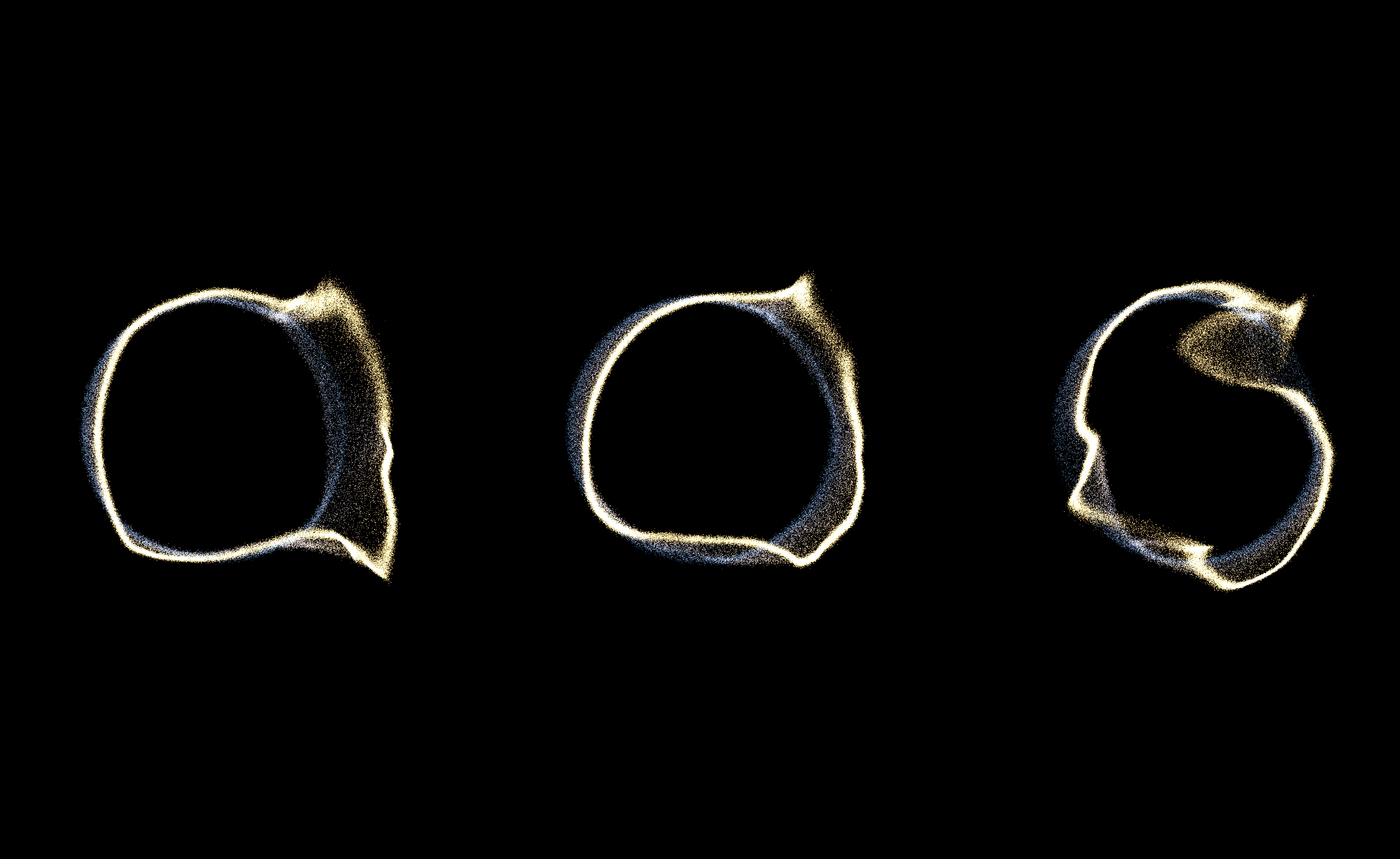
Those are t = 0.25, 0.5 and 0.78 between a "C" and an "S", and none of them is a C, an S,
or a blend of the two. The outer two show a ring with the S's spine pressing into it, before it has
finished being a ring.
The interpolation seals the C into a closed ring and re-opens it the other way; it never slides the C's mouth shut. The middle panel is that ring, and it is the tidiest shape in the sequence: walked in source order, its landing cloud measures about 0.6 of a letter's perimeter, shorter than either endpoint, because a circle is the shortest closed curve there is.
What blendWith needs from the two fields
The same source cloud. Both fields must be trained from one shared cloud, so a particle
has one start point and two destinations. That is also what makes the two normalisation frames
agree, and the API enforces it: blendWith refuses to blend fields normalised
differently, because t = 1 meaning "B's weights read in A's coordinates" is a different field
from B and would look exactly like an interesting result.
The seed matters less than you would expect. Hidden units are exchangeable, so two runs
from different random starts could represent similar functions through different permutations
of the same machinery, and averaging across a permutation would produce nothing. For letters
trained with PAIRED coupling from a shared source, it does not happen: midpoints of fields
trained from different seeds are as tidy as those from one seed, because the two training
problems are nearly the same problem. blendWith does not check seeds. For a wider network,
harder targets or another coupling, train both with the same seed to be safe.
The letter_interpolation starting point sweeps t
slowly and continuously, forty seconds there and back, and
letter_interpolation_panels is the still above. Both need letters that are a single
closed contour in the typeface: C, S, E, F, L, T, V, Z and so on. An O or a D has two, and one
circle cannot be paired with two contours at once.
4. The neighbour grid
Tier two needs a sum over nearby particles, which needs a sort. GpuNeighbourGrid is that, and
it is useful on its own for anything that needs neighbours on the GPU:
val grid = GpuNeighbourGrid(
    capacity = 12_000,
    cellsPerSide = 32, // cellSize = domainSize / cellsPerSide = 0.0625
    domainMin = Vector2f(-1f, -1f),
    domainSize = 2f,
)

// Positions are read as a flat float array: particle i's x is at i * strideFloats + offsetFloats,
// so the grid never needs to know what else is in your struct.
grid.install(renderer.renderList, myParticles, count, strideFloats = 8, offsetFloats = 0)
ShaderBoids calls install for you; you need it only when putting the grid under something of
your own.
Four steps, each avoiding something a compute shader cannot cheaply do:
- hash: one invocation per particle writes
key = cell index,value = particle index. - sort:
GpuRadixSortsorts the pairs, so a cell's members become a contiguous run. This turns a scatter problem into a gather problem. - ranges: one invocation per sorted entry compares its key with its neighbours' and writes each run's bounds. No atomics: an entry can tell whether it begins a run by looking left.
- read: a consumer walks the 3x3 block of cells around its own.
Cells are row-major rather than Morton-ordered. A hierarchy needs a node's children contiguous; a flat grid needs a cell's members contiguous, and row-major does that while making the nine indices of a 3x3 neighbourhood plain arithmetic instead of a bit interleave.
The 3x3 block covers one cell width, so cellSize (domainSize / cellsPerSide) is the largest
radius the query answers correctly. install refuses a larger radius, and one raised past it later
is held to cellSize with a warning in the log. Size the grid from the radius, not from the
particle count.
Particles outside the domain are clamped into the edge cells rather than dropped, because a lost particle is a particle that silently stops interacting.
The whole thing installs as one entry rather than four, because ComputeTarget.render runs every
module before any other consumer, so four separate installs would interleave. If you build
something like it, install once rather than once per module.
5. Boids on the grid
ShaderBoids runs classical Reynolds boids, with its three terms, on top of that grid:
val written = ShaderBoids(grid, count = 12_000) {
    containment = 1.5f
    containmentRadius = 0.44f // a soft wall, applied after the rule
    driverStrength = -0.9f // negative: flee the driver
}
written.installDrawInto() // defaults to renderer.renderList
The default weights flock at this density and radius = 2f / 64f. They are far from the textbook
0.02 / 1.2 / 0.8, which gives an evenly spaced gas here, because separation sums over
neighbours while alignment and cohesion take means. In this scene a boid has about 57
neighbours, and the textbook numbers put separation 27x above alignment and 4600x above cohesion.
If you change radius or the particle count, retune all three. Bring the three terms to the
same order rather than adjusting the weights until it looks right.
separationRadiusFraction is the other dial that decides the shape. One radius for all three terms
cannot clump: separation wants to be short-range while alignment and cohesion want the whole
neighbourhood. Shrinking separation's reach to a quarter turns one even disc into groups.
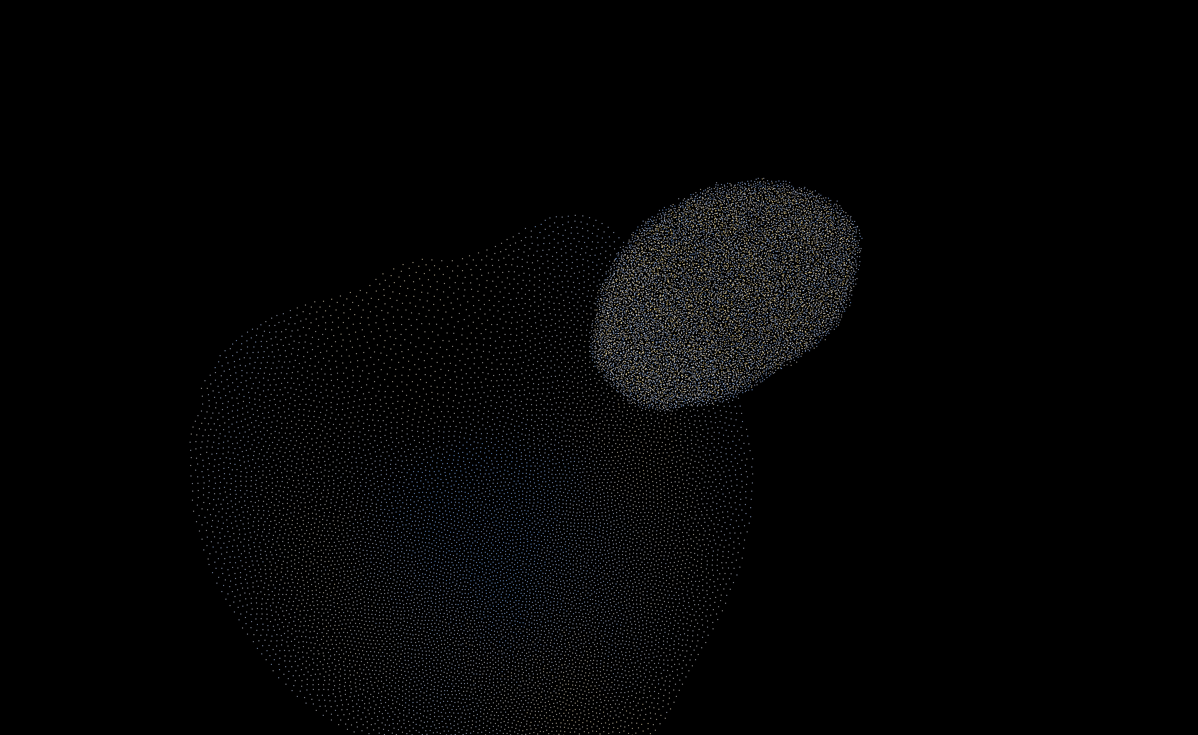
Two flocks of 12,000 at the default weights, with nothing driving them, after a few seconds:
separationRadiusFraction = 1 on the left spreads into one wide, evenly spaced disc that overruns
its soft wall; 0.25 on the right packs into a dense, grainy clump. Undriven, this run did not split
the clump into separate groups.
ShaderBoids works on its own as a fast flocking system. Its force also generates tier two's
training data and is what the learned rule is compared against, which is why it is a written rule
rather than recorded motion: recorded motion would leave nothing exact to compare against.
6. A learned interaction
A velocity field is blind to the other particles. An interaction reads them, and Field fits one with Deep Sets, a network that takes a set of neighbours of any size:
a_i = phi( v_i, SUM_j psi(x_j - x_i, v_j - v_i), MEAN_j psi(...) )Two small networks and a reduction. The aggregation is permutation-invariant and takes any number
of neighbours, so one set of weights serves a particle with three neighbours and a particle with
three hundred. Classical Reynolds is one particular choice of psi and phi, so the family
contains at least one good answer.
Both the sum and the mean are fed to phi, because one reduction is not enough. Separation is
a sum (being crowded by twenty neighbours pushes harder than by two) while alignment and cohesion
are means. Feeding both is worth a factor of four.
Training is one call. You supply a batch of InteractionExample, each a velocity, a list of
neighbours, and the acceleration the rule you are imitating produced. Because you have the rule,
no simulation is needed to generate them:
fun sample(): InteractionExample {
    val v = /* a random velocity */
    val neighbours = /* up to 70 of them, as (dx, dy, dvx, dvy) */
    return InteractionExample(v, neighbours, reynoldsForce(v, neighbours))
}

val learnedRule = trainEquivariant(
    radius = radius, velocityScale = velocityScale,
    accelScale = 20f, sumScale = 8f, minSeparation = minSeparation,
    options = DeepSetsOptions(steps = 4000, batch = 16, seed = 5,
                              psiHidden = intArrayOf(8, 8), messageWidth = 4),
) { List(16) { sample() } }

val learned = ShaderBoids(grid, count = 12_000, equivariant = learnedRule) { /* same settings */ }
learned_boids has this written out in full, with the Reynolds force inline.
Train on the density you will run at
Draw up to seventy neighbours, not a handful. A flock runs at around fifty-seven neighbours per boid once cohesion has gathered it, and a model trained only on sparse neighbourhoods is extrapolating when it runs. That hurts here, because cohesion is weighted against the mean offset, so a small error in the meaned branch becomes a large force.
trainDeepSets and trainEquivariant fit by reverse-mode autodiff over ADTape, because Smile's
MLP cannot express a gradient flowing back through a sum over a variable-length set with shared
weights. Both halves of either form come out as ordinary MlpWeights, so the GLSL emitter from
section 1 applies to them unchanged.
Prefer trainEquivariant. The true rule satisfies a(R x) = R a(x) identically, and nothing in
the plain Deep Sets form makes it do so: a network with scalar weights on Cartesian components has
a preferred direction baked in by its initialisation. The symptom is a flock that drifts steadily in
one direction, and the residual grows with crowding because it rides on the aggregated message.
EquivariantWeights removes it by construction: psi sees only invariants of a neighbour and emits
scalars, the vectors come from the neighbour's own direction and velocity difference, and phi sees
only the lengths of the aggregates. Rotate every input and nothing any network sees changes.
Constraining it this way also improved the fit, which is the usual result when a symmetry is real.
ShaderBoids runs either rule, branching only where the force is computed. The buffer, neighbour
search, integration and speed limit are shared, so two flocks side by side differ only in the
rule:
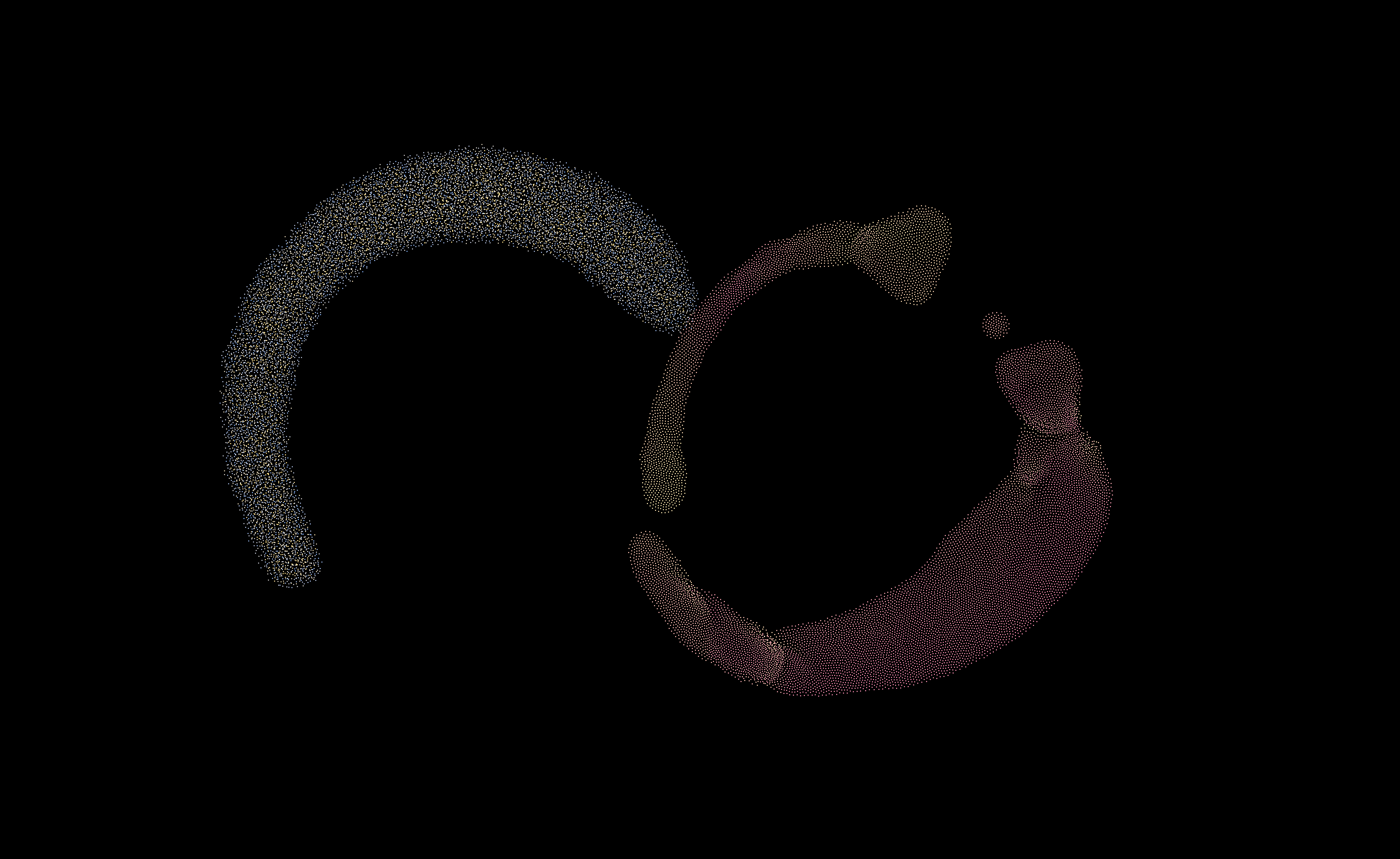
Left is the written rule, right the learned one, twelve thousand boids each, seeded from the same random draw into their own halves of the domain, both fleeing a point that wanders on the same smooth random walk about each flock's own centre.
The learned force has a relative error of about a quarter. That gives a flock that behaves like boids, and over ten thousand chaotic steps the two flocks never look the same.
Retrain after editing the written rule
The learned flock follows the rule as it was when you trained it. Re-run the training box to catch it up; it takes a few seconds. Leaving the two out of step on purpose is how you see how far they can be pulled apart.
Cost
Cost is per neighbour, not per particle, and the learned rule pays a psi forward pass for each
one. Once cohesion has gathered the flock, a boid can have a hundred or more neighbours inside its
radius. At 12,000 boids a flock:
| Configuration | frames per second |
|---|---|
| the written rule alone | 116 |
a 16x16 psi, message width 6 |
17.6 |
an 8x8 psi, message width 4 |
71.2 |
the equivariant 8x8, both flocks, driven |
77 |
The written flock runs at the same speed on the same grid whatever psi is doing, so the cost is
in psi, and tuning cells or particle counts will not help. Keep the depth: a single hidden layer of 16 costs more than two of 8 and
fits worse than either.
7. The driver
With the symmetry built in and no external forcing, the flock settles into something that reads as static: an evenly spaced disc that barely changes. That is what the rule does on its own here; the drift of the plain Deep Sets form was what made it look lively. To get motion, add it from outside the interaction:
boids.settings.driverStrength = -1.5f // negative flees, positive pursues
boids.settings.driverRadius = 0.25f
boids.driver = {
    wanderingPoint()
} // read once a frame
driverStrength adds a pull toward, or a push away from, a point you supply each frame. It is
applied after the rule exactly like containment, defaults to zero, and the network knows nothing
about it, so two flocks side by side still differ only in their rule. No retraining is needed to add or change it.
Settings
NeuralParticleSettings — tier one:
| Setting | Default | Effect |
|---|---|---|
particleCount |
200,000 | Sets the allocation and dispatch size at construction; it cannot be increased on a live system. A few hundred thousand particles is a useful starting scale. |
stepsPerCycle |
150 | Sets frames per source-to-target journey, coupling integrator accuracy to animation speed. Below roughly 60 steps, the target can visibly lose corners. |
dwellCycles |
3 | Holds particles at the target for this multiple of travel time. At three, particles spend three quarters of their cycle on the target. |
phaseSpread |
1 | Spreads initial phases over this fraction of a cycle: one gives a continuous stream and zero a synchronized morph. Call reset() after changing it. |
arrivalBias |
0.8 | Weights brightness toward the end of the journey, from zero to one. Raise it to emphasize the learned target over travelling particles. |
sourceJitter |
0.02 | Adds spread around each source point during reset. Call reset() after changing it; excessive jitter blurs the source correspondence. |
randomSeed |
1 | Controls initial source assignments and particle phases. Reset with the same seed to repeat the initialization. |
viewScale, viewCenter |
2.6, origin | Frame the cloud in normalized training coordinates. Scale controls the visible extent and centre controls the point the view is centred on. |
flipY |
true | Flips the displayed vertical axis. The default accommodates glyph contours, whose y coordinate increases downward. |
pointSize |
1.5f |
Sets the drawn point size in pixels. This changes the appearance without changing the simulated positions. |
sourceColor, targetColor |
(0.15, 0.45, 1, 1), (1, 0.62, 0.22, 1) |
Sets RGBA colours at the beginning and end of each journey. The shader blends between them as the particle travels. |
intensity |
0.5f |
Scales brightness under additive blending. Use it as exposure when overlapping particles make the cloud too bright. |
BoidSettings — tier two. radius must not exceed the grid's cellSize:
| Setting | Default | Effect |
|---|---|---|
radius |
2/64 | Sets the neighbour interaction radius in simulation coordinates. It must not exceed the spatial grid’s cell size, or the query would miss neighbours. |
separation, alignment, cohesion |
0.02, 3, 200 | Weights repulsion, velocity matching and attraction to neighbours’ centre respectively. The defaults flock at about 12,000 boids over a unit square at the default radius; their balance depends on density, so retune them if you change either. |
separationRadiusFraction |
0.25 | Sets separation’s reach as a fraction of radius. Values below one let longer-range cohesion gather clumps without equally long-range repulsion. |
minSeparationFraction |
0.05 | Floors pair distance in the separation denominator at this fraction of radius. This keeps coincident or nearly coincident neighbours from producing unbounded force. |
maxSpeed |
0.25 | Caps speed after acceleration is applied. This keeps one strong interaction from sending a particle arbitrarily far in the next step. |
dt |
1/60 | Sets the fixed integration time step. Set zero to calculate accelerations without moving the particles. |
containment, containmentRadius, containmentCenter |
0, 0.8, origin | Adds a soft restoring force outside a circle centred on containmentCenter. Strength zero disables it; the radius sets where the force begins. |
driverStrength, driverRadius |
0, 0.25 | Controls the moving driver’s force and influence radius. Positive strength attracts and negative strength repels; zero disables the driver. |
pointSize |
2f |
Sets the drawn point size in pixels. This changes the appearance without changing the simulated positions. |
slowColor, fastColor |
(0.16, 0.40, 0.95, 1), (1, 0.75, 0.25, 1) |
Sets the RGBA colours at the low and high ends of the speed tint. This lets the drawing reveal velocity changes without a CPU readback. |
intensity |
0.9f |
Scales brightness under additive blending. Use it as exposure when overlapping particles make the cloud too bright. |
Agents: smoke tests
The four GPU smokes that check this machinery, and what each compares, are listed in
dev_docs/NEURAL_PARTICLES_MEASUREMENTS.md.
Limits
- The learned rule cannot predict the equilibrium residual. In a settled flock, separation and cohesion are large and nearly cancelling, and what survives is a small difference of big terms. Scored on a settled flock, the learned rule does only a little better than predicting exactly zero, and its forces come out about half the size they should be. On scattered neighbourhoods like the ones it was trained on, it is far closer.
- A flock that behaves like boids is not boids, and the picture cannot tell you how close the learned rule is. Compare its forces against the written rule instead.
See also
Flow matching is the CPU half of tier one and worth reading first. Field 4 Graphics is the compute-then-draw shape both systems are built on. The API is in Machine learning and Simulation.
Where the numbers come from
The measurements quoted on this page are in dev_docs/NEURAL_PARTICLES_MEASUREMENTS.md. The
figures are screenshots of the live system, because the native window capture takes stills
only.