Merge trees and contour trees

Slice a landscape at a height and you get islands: the places above that height. Raise the cut and islands shrink, split in two and vanish. Lower it and they grow and join. A contour tree records all of that as one drawing: every island that ever exists is an arc, born at a peak (or a pit), splitting or joining at a saddle. It is the shape of a field's topography with the geometry taken out, and it is often the most legible summary of a field there is.

This example builds a landscape of hills and hollows, computes its contour tree, and shows three things side by side: the field with the tree's nodes marked, the field divided into the regions the tree's arcs stand for, and the tree itself drawn as a plot, with height going up:

import afield.geometry.topology.trees.*

// Seven hills and three hollows.
val bumps = [
    Triple(40.0, 40.0, 1.0),
    Triple(150.0, 35.0, 0.8),
    Triple(100.0, 80.0, 0.6),
    Triple(30.0, 120.0, 0.7),
    Triple(170.0, 120.0, 0.9),
    Triple(120.0, 130.0, 0.5),
    Triple(70.0, 60.0, 0.45),
    Triple(100.0, 30.0, -0.5),
    Triple(60.0, 100.0, -0.4),
    Triple(150.0, 80.0, -0.45),
]
val field =
    Img.generate(200, 150) { x, y ->
        bumps.sumOf { (cx, cy, a) -> a * exp(-((x - cx).pow(2) + (y - cy).pow(2)) / 300.0) }.toFloat()
    }

// Simplifying (below) prunes the many tiny branches shorter than 0.03.
val tree = ContourTrees.contourTree(field).simplify(persistence = 0.03)
val dots = fline {
    tree.nodes.forEach { moveTo(it.x, it.y) }
    pointed = true
    pointSize = 5.0
}
val plot = Img(200, 150, 3, FloatArray(200 * 150 * 3)).drawFLines(tree.plot(200.0, 150.0, margin = 15.0), scale = 2.0)
showImgGrid(
    "field: ${tree.nodes.size} nodes" to
        field.normalized().colormap("viridis").drawFLines([dots], scale = 2.0, color = Vec4(1f, 1f, 1f, 1f)),
    "regions: ${tree.arcs.size} arcs" to tree.segmentationImage().scaleBy(2.0),
    "tree" to plot,
    columns = 3,
    cellSide = 300,
)

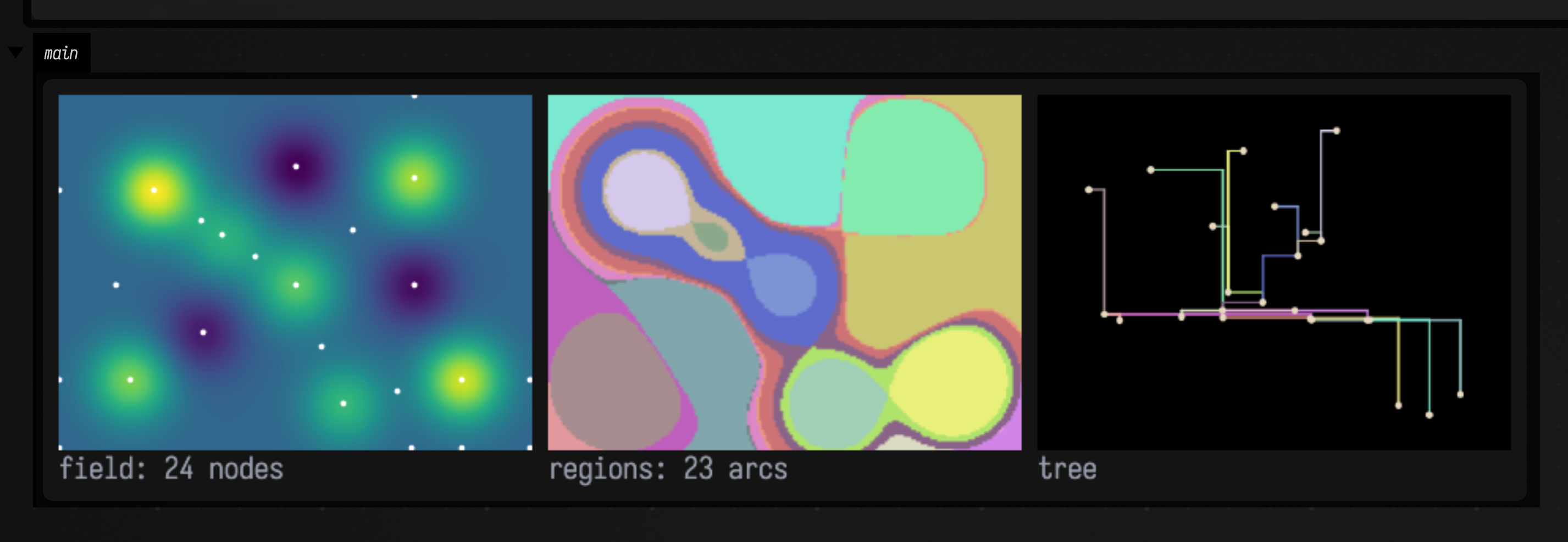
Every peak is a leaf at the top of the plot and every pit a leaf at the bottom; branches meet at saddles, at the height where two islands (or two lakes) touch. The coloured regions are the same arcs on the ground: each region is the set of places whose contour line belongs to that arc. The dots on the frame's edge are real as well: the field is cut off there, so the edge has low points and saddles of its own.

Join trees and split trees

The contour tree is built from two simpler trees. The join tree (ContourTrees.joinTree) floods the landscape from below: a lake starts at every pit, lakes join at saddles, and everything is one lake when the water passes the highest point. The split tree (ContourTrees.splitTree) does the same from the top down, with islands. Each sees only half the story: the join tree records joins and the split tree splits. ContourTrees.contourTree merges the two by Carr, Snoeyink and Axen's method (2003), peeling off one leaf at a time, so it records both.

import afield.geometry.topology.trees.*

// Seven hills and three hollows.
val bumps = [
    Triple(40.0, 40.0, 1.0),
    Triple(150.0, 35.0, 0.8),
    Triple(100.0, 80.0, 0.6),
    Triple(30.0, 120.0, 0.7),
    Triple(170.0, 120.0, 0.9),
    Triple(120.0, 130.0, 0.5),
    Triple(70.0, 60.0, 0.45),
    Triple(100.0, 30.0, -0.5),
    Triple(60.0, 100.0, -0.4),
    Triple(150.0, 80.0, -0.45),
]
val field =
    Img.generate(200, 150) { x, y ->
        bumps.sumOf { (cx, cy, a) -> a * exp(-((x - cx).pow(2) + (y - cy).pow(2)) / 300.0) }.toFloat()
    }

:::fold draw the three trees
// The two halves and their merge, each simplified the same way and drawn as a plot.
fun drawn(tree: ScalarTree) =
    Img(200, 150, 3, FloatArray(200 * 150 * 3)).drawFLines(tree.simplify(persistence = 0.03).plot(200.0, 150.0, margin = 15.0), scale = 2.0)
showImgGrid(
    "join tree" to drawn(ContourTrees.joinTree(field)),
    "split tree" to drawn(ContourTrees.splitTree(field)),
    "contour tree" to drawn(ContourTrees.contourTree(field)),
    columns = 3,
    cellSide = 300,
)

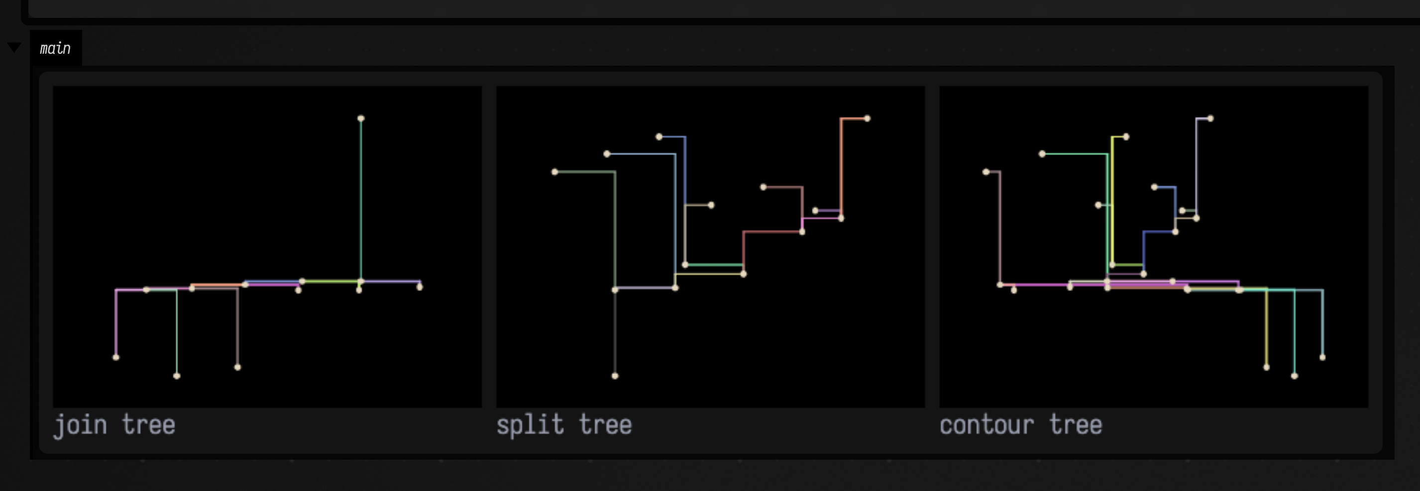
The join tree has a leaf for every pit and a single top; the split tree has a leaf for every peak and a single bottom. Only the contour tree has both.

Use a merge tree on its own when only one direction matters: the split tree of a density map is the hierarchy of its clusters, and the join tree of a distance field is the hierarchy of its basins.

Simplifying

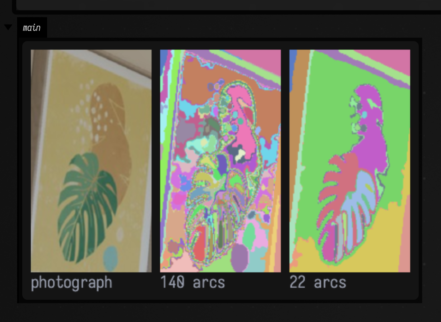
A field with any noise has a tree with thousands of tiny branches, one for every speck. tree.simplify(persistence) removes leaf arcs shorter than persistence (in the field's units, from leaf to saddle) one at a time, smallest first, and gives their pixels to the branch they hung from. It is the same persistence that simplifies a Morse–Smale complex: small bumps go first and the large structure stays.

This example takes the brightness of a photograph of a printed leaf, cropped from one of the docs' own pictures, and simplifies its contour tree twice:

import afield.geometry.topology.trees.*

val print = imgFromFile("public/docs/assets/vision/fline-viewer.jpg", 3).crop(78, 262, 128, 236)
val tree = ContourTrees.contourTree(print.luma().gaussianBlur(1.5))
val light = tree.simplify(persistence = 0.01)
val strong = tree.simplify(persistence = 0.05)
showImgGrid(
    "photograph" to print.scaleBy(2.0),
    "${light.arcs.size} arcs" to light.segmentationImage().scaleBy(2.0),
    "${strong.arcs.size} arcs" to strong.segmentationImage().scaleBy(2.0),
    columns = 3,
    cellSide = 260,
)

What you get

A ScalarTree has nodes (each a TreeNode with its pixel position, value and type: MINIMUM, MAXIMUM, SADDLE, or ROOT for the end of a merge tree) and arcs (each a TreeArc from a lower node to an upper one, with the pixels it owns as vertices). arcOfPixel gives every pixel's arc, and arcsAt(node) the arcs meeting at a node.

For drawing, plot(width, height, margin) lays the tree out as FLines, segmentationImage() colours the regions, and network() returns the tree as a GeometryNetwork in image space, nodes carrying their type and value, so it chains into the other geometry tools.