Deep Dive: Force-Directed Semantic Web Visualization in Field 14
Or: How to re-implement RelFinder in an afternoon.
This long page is going to take you through the process of building a small workbench for visualizing and exploring relationships found in semantic web databases. Specifically, we're going to build a completely unpolished, but usable version of RelFinder which is a "graph relationship visualizer". I will also use this exercise as an opportunity to reflect a little about the differences between something like Field and something like RelFinder. Or, for that matter, any other such tool — I'm picking on RelFinder because it's a very masterfully made example of a widely encountered visualization approach. It has gotten to the point where a force-directed graph layout visualization of semantic web data has become a rite of passage for any visualization framework. It's only natural to investigate what it's like to build these things in Field. Fortunately the answer is: very straightforward.
We're going to see a few Field things in action along the way:
- How to draw 2d things directly on the canvas — specifically graphs and text.
- How to add simple mouse behaviors to these things.
- How to include huge 3rd party Java libraries into Field — specifically Jena
- How to hack our way into those libraries without stopping to read or even locate their documentation using auto-completion.
- How to include tiny little class files you write yourself in Eclipse into Field — specifically a force directed layout class.
- How to customize Field's autocompletion — to provide database driven completions.
- How to build and use some simple multi-threading in Field.
I'm going to go over each step of this tutorial in a lot of detail — to cover the use of Field in depth — even if it means backtracking and refactoring our work as we progress towards the goal. This really is the documentation of "an afternoon" working Field towards a particular implementation. Each step will have a downloadable .field sheet that you can use to play with if you don't want to copy and paste the code from this browser or are unclear what code goes where.
Where are we going?
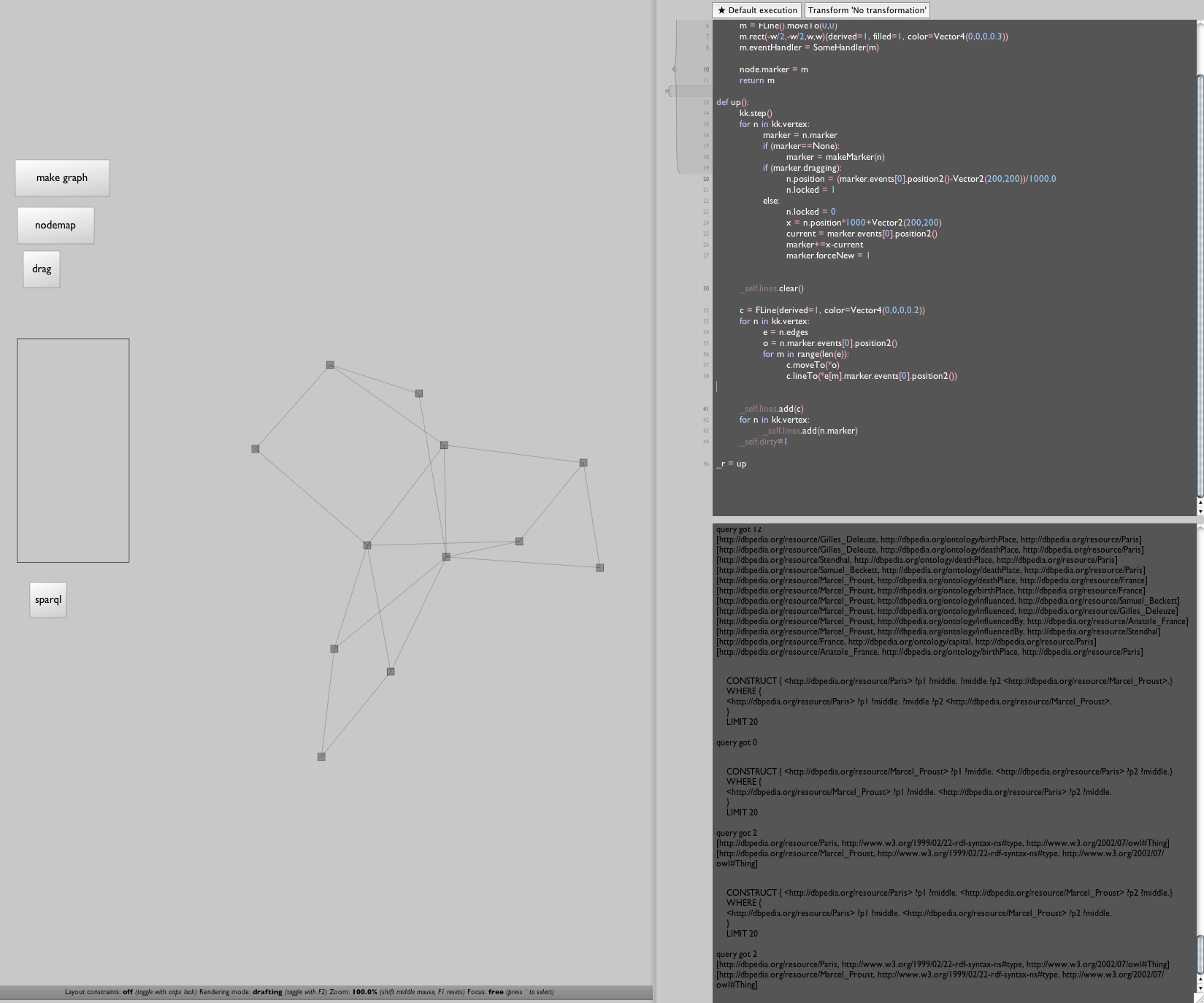
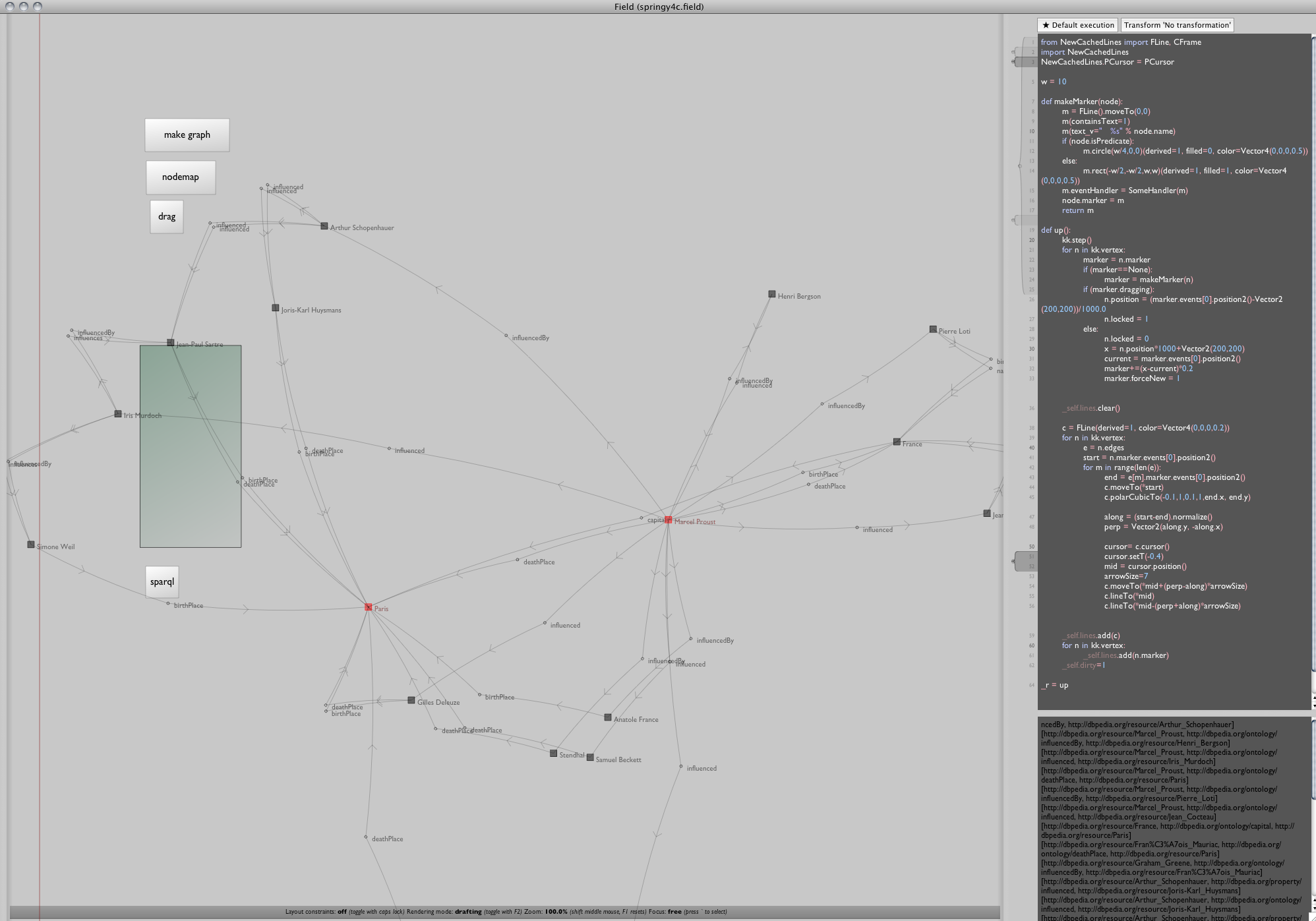
Here's where we are heading:
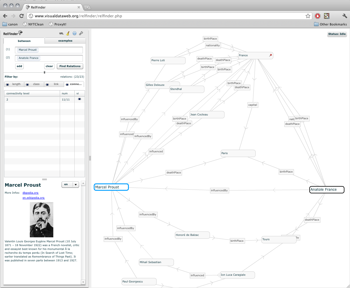
(all images on this page can be expanded by clicking on them)
There's a graph on the right showing a network of nodes connecting "Marcel Proust" and "Anatole France". More technically speaking, a network of nodes connecting <http://dbpedia.org/resources/Marcel_Proust> and <http://dbpedia.org/resources/Anatole_France>. These relationships have been built up by successive queries — submitted using the SPARQL query language — against dbpedia.org (a large RDF database containing semantic web data mined out of wikipedia).
This network is the force directed layout part — those nodes that repel each other (slightly) and the edges that connect the nodes are a little like springs (they want to be a certain length). Typically after 30 or so nodes have appeared on screen everything turns into a bit of a mess, but crucially you can still drag the nodes around with the mouse to flatten out parts of the graph that you are interested in.
On the left is the UI for choosing what nodes to start with (Proust and France) and what kinds of edges and nodes to show and hide. We're going to mimic, Field style, each of these things.
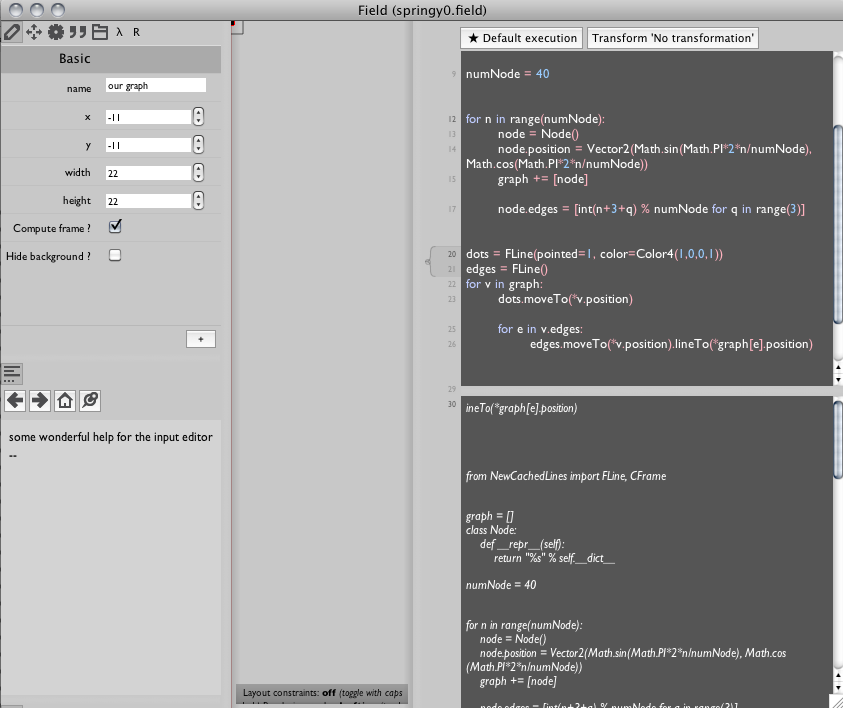
Step 1a: Let's draw a graph
Download the code for this step here.
Let's start at the very beginning: let's draw a graph in Field. To draw something (and to write the code to draw it) we need a place to put it — a "new spline drawer" (from the right-click menu on canvas, or the shortcut "P").
This blank box will automatically move to be near anything that we draw in it.
Now the world's most simple graph data-structure:
graph = []
class Node: pass
That's it! We'll exploit the fact that Python classes are open (you can stick anything you like in them). We'll use anode.edges # [...] to store the edges and someOtherNode.id 4 to store their names. Actually, here's a tip: a better graph data-structure is this:
graph = []
class Node:
    def __repr__(self):
        return "%s" % self.__dict__
This is the world's second-most-simple graph data-structure — this will helpfully print out everything that's in it when we ask it to. Since Field encourages you to be constantly print'ing the contents of variables it's nice when they have good __repr__ methods (in Python) or toString() methods (in Java).
Now we need some nodes:
numNode = 40
for n in range(numNode):
    node = Node()
    node.position = Vector2(Math.sin(Math.PI*2*n/numNode), Math.cos(Math.PI*2*n/numNode))
    graph += [node]
We've added a .position property to them. Vector2 is a class built into Field and when we say Math.sin we're really referring to the one built into Java.html).
Of course, it's not really a graph until we have some edges. So lets add:
node.edges = [int(n+3+q) % numNode for q in range(3)]
That's just going to connect each node to three others further along in the circle. Anything just to get started.
Now to plot them:
# red vertices
dots = FLine(pointed=1, color=Color4(1,0,0,1))
# black (default) edges
edges = FLine()
for v in graph:
    dots.moveTo(*v.position)
    for e in v.edges:
        edges.moveTo(*v.position).lineTo(*graph[e].position)
_self.lines.clear()
_self.lines.add(dots)
_self.lines.add(edges)
FLine() creates a new container for drawing; _self.lines.add(...) adds it to the list of things that this code box draws. But triumphantly executing all of this might yield confusion — in fact, you might wonder where your code box has gone. Careful inspection shows that it has all bit disappeared up to the top left of the canvas:
(it's that red dot). Of course, our graph node .position properties all fit within the unit circle which, when we draw it with the default zoom, is one whole pixel wide. We need to scale and translate that up so we can actually see it:
# red, big dots for vertices
dots = FLine(pointed=1, pointSize=10, color=Color4(1,0,0,1))
# black translucent edges
edges = FLine(color=Color4(0,0,0,0.3))
for v in graph:
    dots.moveTo(*v.position)
    for e in v.edges:
        edges.moveTo(*v.position).lineTo(*graph[e].position)

dots *= CFrame(s=200, t=Vector2(300,300), center=Vector2())
edges *= CFrame(s=200, t=Vector2(300,300), center=Vector2())

_self.lines.clear()
_self.lines.add(dots)
_self.lines.add(edges)
CFrame (short for coordinate frame) transform drawn material here by scaling it up and translating it around a center; yielding:
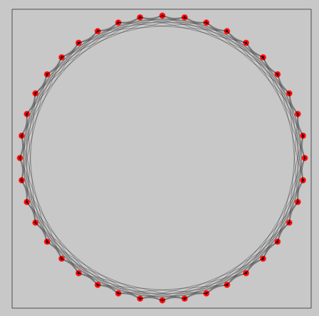
Exactly what we'd expect.
Exercises
- You can stop here and play around with the graph topology and the original
.positionassignments to create new shapes to make sure that you understand the drawing coordinate systems. FLineoffers a pretty rich collection of drawing functions — take a close look at the documentation and create some more elaborate drawings of these graphs. In particular we are not drawing the edge direction (yet).
Step 1b. Drag something around
Download the code for this step here.
That's the first part of the puzzle. But this drawing neither animates — it is not "force-directed" — nor is it interactive — you can't drag anything around with the mouse. Let's fix this. Field can add code to lines and this code is called when the lines are moused over, clicked on or dragged. This lets you manufacture buttons and sliders and so on out of whole cloth.
Full documentation can be found here, but we just need a draggable box for our nodes. First a rectangle:
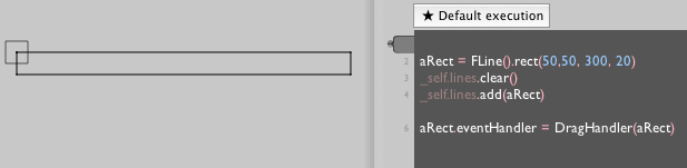
To add behavior to it, we need to add an .eventHandler to it:
class DragHandler(Eventer):
        def __init__(self, line):
                Eventer.__init__(self)
                self.on= line

        def down(self, event):
        self.downAt = Vector2(event.x, event.y)

    def drag(self, event):
        self.on+=Vector2(event.x-self.downAt.x, event.y-self.downAt.y)
        self.downAt = Vector2(event.x, event.y)
        return 1 # returning 1 means that we need to redraw the canvas

aRect.eventHandler = DragHandler(aRect)
Execute that, and that's it: now you have a rectangle that you can drag around with the mouse.
The key line is self.on +# Vector2(...) — the + operator mutates the FLine here by translating it by how much the mouse has moved.
Exercise
- By setting (and restoring) the color property on
self.onimplement a change of color on mouse down / up and hover just like buttons normally have. You'll need to addup(...),enter(...)andexit(...)methods to your callback.
Step 1c. A Force directed layout
Download the code for this step here.
Now we need a force directed layout algorithm. We could write one ourselves here, the simple ones are certainly easy enough. But truth be told I cannot bear it. A force directed graph demo was some of the first Java code I every laid eyes on (version here) some 15 years ago: there's code that you need to write yourself and there's code that you find in a library somewhere.
Besides, while the dumbest graph layout approach is straightforward, the more advanced approaches get quite involved — truly the kind of code you want not to write, but rather have boxed up, ready to swap out for a different approach provided by some other library.
Let's grab something from the JUNG graph library a large repository of graph algorithms (and quite a few layout approaches as well). We'll grab the source (it's under the BSD license) of a Kamada-Kawai implementation so that we can tweak it a bit — in particular I've modified it so that I can dynamically add and remove nodes. This work got done with Field side-by-side with Eclipse (my favorite Java editor) using the reload plugin to continually reload the layout class as I tweaked it to make sure that it was still working. To add arbitrary class files (together with their Java sources) to Field, see these instructions here.
But for the purposes of providing a freestanding, hackable piece of tutorial code, I've included the Java for the layout "engine" inside the tutorial Field sheet — not the .class file, the actual Java source. Field will happily compile it (and let you incrementally edit it). Field comes with support for embedded Java (in addition to other languages).
Ultimately, for our purposes here, the choice of layout code is not our main interest. We care about three things: firstly, the layout class — here called SpringUtilCobj, takes an array of nodes to layout and a distance metric function that captures their connectivity. Secondly, there's a method called step() that moves everything around to layout "just a little bit better" — we'll be calling this every animation frame. And thirdly, any layout algorithm is going to have a few magic "constants" that you are going to have to vary a little to get the best results. Fortunately we'll be varying them in real-time.
First we'll make another random graph, just like before:
from field.graph import SpringUtilCobj
from field.context.Context import Cobj
numNode = 40
graph = []
for n in range(numNode):
    node = Cobj(id=n)
    edges = []
    for q in range(2):
        edges += [int(n+3+q+Math.random()*0.1) % numNode]
    node.edges = edges
    graph += [node]

def metric(x,y):
    if (y.id in x.edges):
        return 0.1
    return -1

# --- this is our layout engine
kk = SpringUtilCobj(metric, graph)
Our metric function here is very obvious — if two nodes are connected, then the distance between them should be 0.1. Otherwise return '-1' to say that they are not connected.
We've switched from our trivial Node class to a standard Field Cobj class — they happen to have nicer interfaces from Java. Had we found a graph layout algorithm that had a particularly strong opinion about its node class we'd be using that instead.
If we leave our drawing code unchanged:
# red, big dots for vertices
dots = FLine(pointed=1, pointSize=10, color=Color4(1,0,0,1))
# black translucent edges
edges = FLine(color=Color4(0,0,0,0.3))
for v in graph:
        dots.moveTo(*v.position)
        for e in v.edges:
                edges.moveTo(*v.position).lineTo(*graph[e].position)

dots *= CFrame(s=200, t=Vector2(300,300), center=Vector2())
edges *= CFrame(s=200, t=Vector2(300,300), center=Vector2())
_self.lines.clear()
_self.lines.add(dots)
_self.lines.add(edges)
we get:
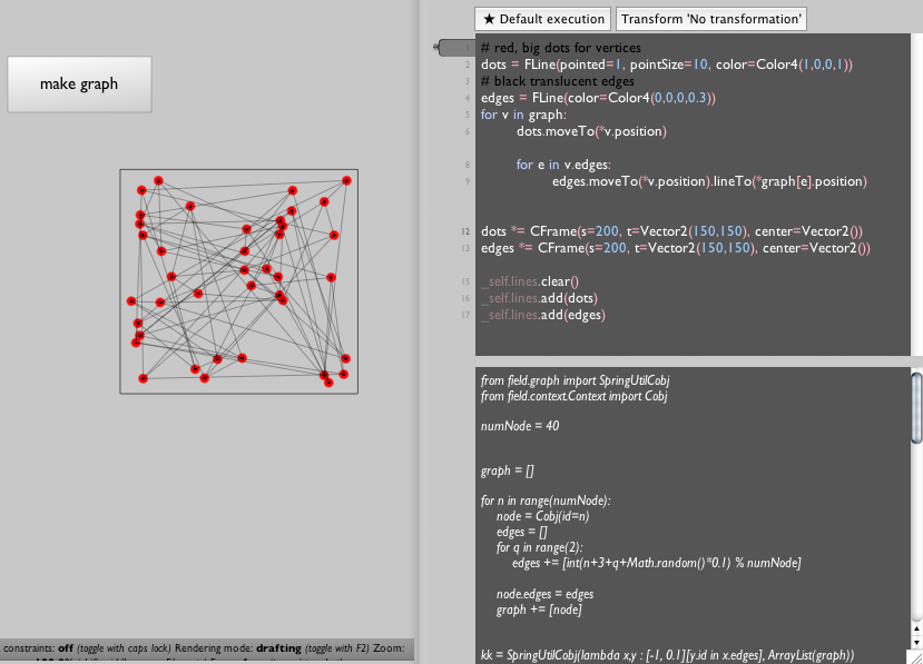
Note one refactoring: I've moved the graph creation code out to its own box, away from the graph drawing code — you can create a new box from the contextual menu on the canvas. This makes sense because our next move will be to create the graph once and then draw it many times.
Animation in Field means calling a set of functions over and over again — once per animation frame. Field has a concept of starting, running, stopping (and pausing) a box.
To tell Field what we want to do when this box is "run" we modify our drawing routine slightly:
def animate():
    # --- call the graph layout code
    kk.step()
    # --- tell field to redraw the canvas
    _self.dirty=1
    # --- draw the nodes and edges
    dots = FLine(pointed=1, pointSize=10, color=Color4(1,0,0,1))
    edges = FLine(color=Color4(0,0,0,0.3))
    for v in graph:
            dots.moveTo(*v.position)
            for e in v.edges:
                    edges.moveTo(*v.position).lineTo(*graph[e].position)

    # --- scale everything to be visible
    dots *= CFrame(s=200, t=Vector2(150,150), center=Vector2())
    edges *= CFrame(s=200, t=Vector2(150,150), center=Vector2())

    # --- tell Field to associate these FLines with this box on the canvas
    _self.lines.clear()
    _self.lines.add(dots)
    _self.lines.add(edges)

# --- declare that to "run this box" means to call animate over and over again
_r = animate
We are free to "start" and "stop" boxes in Field using a variety of techniques (command-page up, option clicking, using time-lines, and even using code in other boxes) — see VisualElementLifecycles for a complete list.
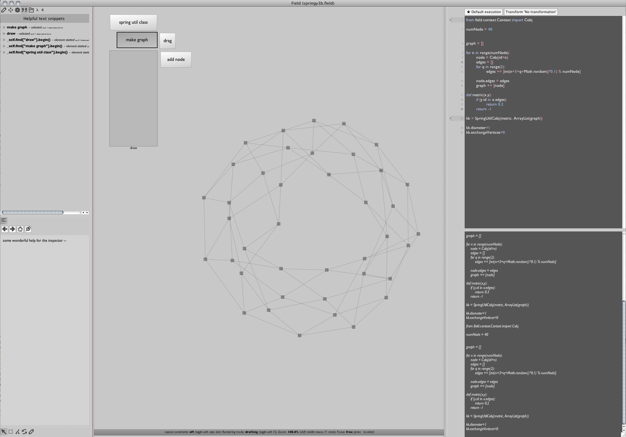
Now after a few seconds of animation we have something like:
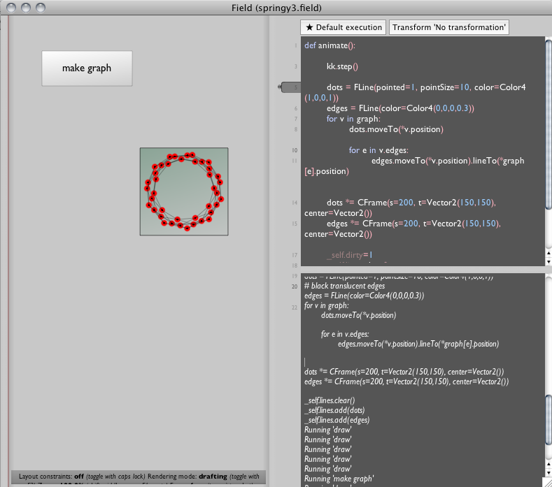
That seems good, but a little compact, so we start tweaking the distance metric in "make graph":
def metric(x,y):
    if (y.id in x.edges):
        return 0.1
    return -1
becomes:
globalEdge=0.1
def metric(x,y):
    if (y.id in x.edges):
        return globalEdge
    return -1
And we execute all of the "make graph" box again (command-zero is a handy shortcut for this). We do this even while our main graph visualizer is still animating. Immediately it snaps back to a random graph. But now we can modify the value of globalEdge without resetting anything.
Changing this number does indeed change the compactness of the graph. At globalEdge=0.3:
If this was a particularly important number (or if it had a few friends all needing experimentation) I might replace it in the text editor with a slider:
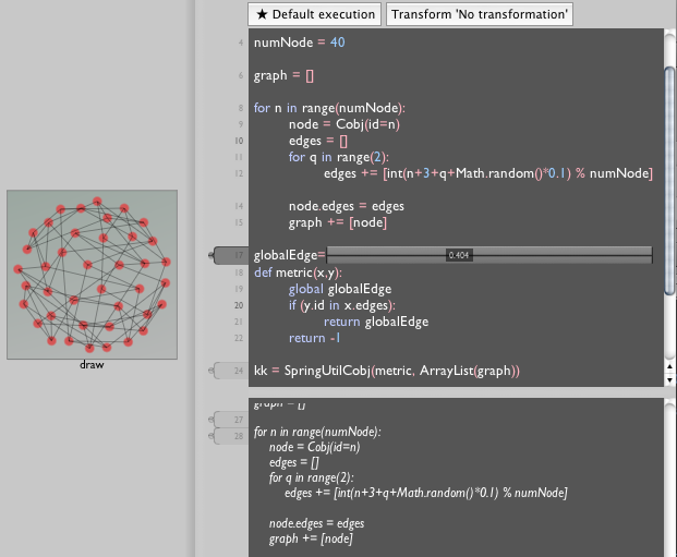
Field supports a number of text-editor embeddable GUI widgets that take some of the burden out of writing code while still compiling down to text.
Exercise
- Go Google yourself another single class graph layout algorithm and refactor this step of the tutorial to use that one instead.
Step 1d. Putting it all together
Download the code for this step here.
We have graph drawing, we have interaction, we have force-directed layout: let's refactor each of these things slightly and put all these things together.
First our DragHandler becomes:
class DraHandler(Eventer):
        def __init__(self, line):
                Eventer.__init__(self)
                self.on= line
        def down(self, event):
        self.downAt = Vector2(event.x, event.y)
        self.on.dragging = 1
                return 1
        def up(self, event):
        self.on.dragging = 0
                return 1
    def drag(self, event):
        self.on+=Vector2(event.x-self.downAt.x, event.y-self.downAt.y)
        self.on.forceNew=1
        self.downAt = Vector2(event.x, event.y)
        return 1
Here's we're using the fact that we can store arbitrary properties inside FLine instances ("dragging") to mark lines that are in the process of being dragged around. If the are being dragged around we don't want the graph layout code to update their positions, rather we want to it to go the other way — have the graph layout code's position get updated from the FLine.
Our graph generation code remains the same as before:
from field.context.Context import Cobj
numNode = 40
graph = []

for n in range(numNode):
    node = Cobj(id=n)
    edges = []
    for q in range(2):
        edges += [int(n+3+q+Math.random()*0.1) % numNode]
    node.edges = edges
    graph += [node]

def metric(x,y):
    if (y.id in x.edges):
        return 0.1
    return -1

kk = SpringUtilCobj(metric, ArrayList(graph))
The biggest change is of course the drawing code: this is where the interaction meets the layout.
First we're going to need some markers that can get dragged around — one per graph node. We need a function to make them:
markerWidth = 10

def makeMarker(node):
    m = FLine().moveTo(0,0).rect(-markerWidth/2,-markerWidth/2,markerWidth,markerWidth)
    m(derived=1, filled=1, color=Vector4(0,0,0,0.3))
    m.eventHandler = DragHandler(m)
    node.marker = m
    return m
With this function we'll be able to associate a piece of geometry (an FLine) with a graph node (a Cobj). It makes a filled square (with side markerWidth) centered at the origin.
Now are animation loop looks like this:
def up():
    # ---- the layout step
    kk.step()

    for node in graph:
        marker = node.marker
        if (marker==None):
            marker = makeMarker(node)

        if (marker.dragging):
            # ---- send the position of the geometry to the layout engine
            node.position = (marker.events[0].position2()-Vector2(200,200))/1000.0
            node.locked = 1
        else:
            # ---- send the position of the layout to the geometry
            node.locked = 0
            x = node.position*1000+Vector2(200,200)
            current = marker.events[0].position2()
            marker+=x-current
            marker.forceNew = 1

    # ---- draw everything just like before
    connections = FLine(derived=1, color=Vector4(0,0,0,0.2))
    for node in graph:
        e = node.edges
        o = node.marker.events[0].position2()
        for m in range(len(e)):
            connections.moveTo(*o)
            connections.lineTo(*graph[e[m]].marker.events[0].position2())

    _self.lines.clear()
    _self.lines.add(connections)
    for node in graph:
        _self.lines.add(node.marker)

    _self.dirty=1

_r = up
Let's go through the highlights of this:
if (marker#None): marker = makeMarker(node)—FLines for nodes are made lazily. We're aiming towards being able to add nodes dynamically to out graph, so having geometry get created on demand inside our animation loop is the most convenient way of structuring thisif (marker.dragging): ... else: ...— if the marker is being dragged then we update the node position from marker (and tell the graph layout engine) if it isn't then we go the other way — update the marker from the node position.- __
marker.eventsis the list of control nodes that make up the geometry of a line. You can see from themakeMarkerfunction that we've inserted a.moveTo()event at the center of the marker. Thusmarker.events[0].position2()is the position of the center of the square. marker+#x-current— this moves the marker geometry so that its center is at 'x' — the transformednode.position. If you want the graph to animate more smoothly, simply change this line to bemarker+(x-current)*0.1and the marker will smoothly track towards the graph layout.
The rest of the code is essentially unchanged from previous steps.
With these pieces in place we have a force directed graph layout system that you can interact with:
Exercise
- Implement pinning — this will let you keep a node fixed in place, just as if you were constantly "dragging" it. Hint:
event.count#2will test for a double click in adown(...)callback.
Step 2. Some SPARQL
Download the code for this step here.
We're about half way there — we have the ability to dynamically layout graphs. Now we need some data to drive the creation of those graphs. The storage format of the Semantic Web is RDF and the Query language for querying big RDF stores is SPARQL which is roughly equivalent (and extremely inspired by) SQL. There are plenty of resources about SPARQL online, and besides, I'm certainly not expert. In fact, part of the purpose behind "this afternoon" was to become more familiar with SPARQL and the messy details of real databases. It turns out that by repeated application of autocompletion and by embedding SPARQL in languages that I'm more familiar with Field is a pretty good place to learn SPARQL.
To follow along all you really need to know is this: that semantic web databases are (sometimes huge) collections of triples (object, predicate, subject) that hopefully form interesting graphs of interesting data.
To explore these graphs, first we need to be able to issue and receive SPARQL queries out of Field. It first blush I'm in a position of weakness — I hardly know SPARQL itself, let alone a library to use it, even my SQL is a little rusty. The trick is to execute and inspect everything. Does Field have SPARQL support? No. But Field is based on not one but two of the most promiscuous runtimes in IT today — Java and Python. This means that we're looking for any Java or pure-Python library that provides this task. A moment with Google yields the Jena project — a set of Java bindings that look like‘ they contain what I need; and one internet minute later I'm looking at:
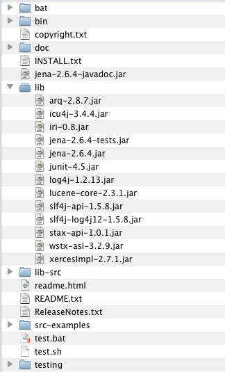
I tell Field about this "lib" directory — in the Plugin manager right-click somewhere and say "add directory full of jars". Go ahead and include lib-src as a Java source jar as well (this improves the auto-completion and documentation that Field can provide). Restart Field and you can now execute the following code:
from com.hp.hpl.jena.query import *
res = QueryExecutionFactory.sparqlService("http://dbpedia.org/sparql",
"""
SELECT *
WHERE {
<http://dbpedia.org/resource/Marcel_Proust> ?p1 <http://dbpedia.org/resource/Paris>.
}
LIMIT 20
""").execSelect()
Roughly, this query asks the DBPedia database for any and all predicates that exist between Marcel_Proust and Paris. Truth be told, I generate this query out of a combination of the SPARQL I do know and running WireShark to intercept RelFinder's conversation with dbpedia.
(Note the first time you run this code might take 5-10 seconds — Field lazily loads 2000 or so classfiles for Jena into the Java virtual machine. Don't panic: subsequent queries are quite fast).
Where did QueryExecutionFactory.sparqlService( ... ) come from? Some example code I found online. Pressing command-I after writing QueryExecutionFactory auto generates the "from ... import ..." form at the top. The point here is that Field is optimized for the speed with which I can audition snippets of code as I explore an alien framework.
Now we have a 'res' object — what to do with it? we could look for some documentation, but better would be just to start hacking our way into it using Field.
First we write:
res
on a line by itself. By pressing commmand-/ we automatically execute print res. This yields:
com.hp.hpl.jena.sparql.resultset.XMLInputStAX$ResultSetStAX@38a4d1fb
Well that wasn't helpful, but it was worth a shot. So next we add a '.' after the res then press command-period to ask Field for some autocompletion help:
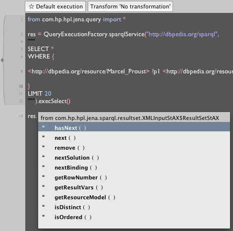
the hasNext() and next() are the clue we need:
while res.hasNext():
    print res.next()
Prints:
( ?p1 = <http://dbpedia.org/ontology/deathPlace> ) -> [Root]
Much more interesting. Next:
while res.hasNext():
    n = res.next()
We rerun the query, because clearly res is some kind of iterator that gets used up once we've next()ed it too much (we don't need to be clairvoyant to know this, not doing this yields an error in Field's output window right away). Saving res.next() to n allows us to get auto-complete on n:
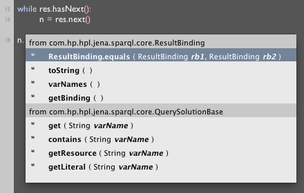
At this point Field has found some source code that it can parse and is providing variable names (doesn't look like there are any JavaDoc's in the source code though, otherwise we'd see them too). I like the look of .get(varName), and sure enough:
while res.hasNext():
    n = res.next()
    print n.get("?p1")
Prints:
http://dbpedia.org/ontology/deathPlace
Marcel Proust did indeed die in Paris; and we've gotten a handle on about half of the SPARQL we need for this project.
Step 2b. Finding relationships
Let's iteratively move towards a fuller set of SPARQL queries. The game here — which you can glean from finding the right paper or by packet capture — is to submit queries with increasingly flexible structure ones which permit more and more intermediate object, predicate and subject triples between our search topics.
Here's where we are:
def runQuery(**kw):
    return QueryExecutionFactory.sparqlService("http://dbpedia.org/sparql",
    """
   SELECT *
   WHERE {

   %(a)s ?p1 %(b)s

   }
   LIMIT 20
   """ % kw).execSelect()

res = runQuery(a="<http://dbpedia.org/resource/Marcel_Proust>", b="<http://dbpedia.org/resource/Paris>")

while res.hasNext():
    n = res.next()
    print n.get("?p1")
Let's refactor that a little more. The bottom expression can become:
while res.hasNext():
    n = res.next()
    print ["%s = %s" % (x, n.get(x)) for x in n.varNames()]
This prints any and all variables that we might SELECT in a query not just ?p1 — varNames() is found and deployed using the techniques above. Once we have that written and tested we wrap it in a function:
proust = "<http://dbpedia.org/resource/Marcel_Proust>"
paris = "<http://dbpedia.org/resource/Paris>"

def printResults(res):
    while res.hasNext():
        n = res.next()
        print ["%s = %s" % (x, n.get(x)) for x in n.varNames()]

printResults(runQuery("%(a)s ?p1 %(b)s", a=proust, b=paris))
Now we have a one line SPARQL test-bench. Quickly we get:
printResults(runQuery("%(a)s ?p1 ?middle. ?middle ?p2 %(b)s.", a=proust, b=paris))
printResults(runQuery("%(a)s ?p1 ?middle. %(b)s ?p2 ?middle.", a=proust, b=paris))
printResults(runQuery("%(a)s ?p1 ?middle1. ?middle1 ?p2 ?middle2. ?middle2 ?p3 %(b)s", a=proust, b=paris))
We can experiment with other URIs for a and b and we can swap them around. But we can tell that they are generating results. Obviously, there is a temptation to stop now and make a function to generate all queries like this under a certain length, but to clear I don't feel like I quite have a handle on the nature of some of the longer topologies.
In particular one thing that we have not added to our queries are any FILTER expressions — we ask for all matches. This is touched upon by the literature, but it remains as far as I can tell at best a dark art and at worst a dirty secret. There are a number of predicates that are, for the ambitions of a "general" tool like RelFinder, deemed hopelessly unimportant — so unimportant that they appear to be filtered out. From packet capture:
FILTER ((?pf1 != <http://www.w3.org/1999/02/22-rdf-syntax-ns#type> ) && (?pf1 != <http://www.w3.org/2004/02/skos/core#subject> ) && (?pf1 != <http://dbpedia.org/property/wikiPageUsesTemplate> ) && (?pf1 != <http://dbpedia.org/property/wordnet_type> ) && (?pf1 != <http://dbpedia.org/property/wikilink> ) && (?pf1 != <http://www.w3.org/2002/07/owl#sameAs> ) && (?pf1 != <http://purl.org/dc/terms/subject> ) && (?ps1 != <http://www.w3.org/1999/02/22-rdf-syntax-ns#type> ) && (?ps1 != <http://www.w3.org/2004/02/skos/core#subject> ) && (?ps1 != <http://dbpedia.org/property/wikiPageUsesTemplate> ) && (?ps1 != <http://dbpedia.org/property/wordnet_type> ) && (?ps1 != <http://dbpedia.org/property/wikilink> ) && (?ps1 != <http://www.w3.org/2002/07/owl#sameAs> ) && (?ps1 != <http://purl.org/dc/terms/subject> ) && (!isLiteral(?middle)) && (?middle != <http://dbpedia.org/resource/Marcel_Proust> ) && (?middle != <http://dbpedia.org/resource/Paris> ) )
This is a big grab-bag of secret knowledge — both domain- and use-specific. Domain-specific because it depends on URIs that DBpedia uses and generic URIs that are used in specific ways by DBpedia; Use-specific because I'll bet there actually are some uses for that Wordnet information out there.
We're going to proceed without explicit FILTER expressions on our queries because, unlike RelFinder we never have to worry about getting too far away from the String where we'd put them in. In any case, paradoxically, I'd need a tool exactly like the one I'm building here to help me write those FILTER clauses in the first place.
Step 2c. Generating graphs from SPARQL results
Download the code for this step here.
Let's have one last refactoring before we turn these SPARQL results over to our graph visualizer. Up until now, we've been issuing SELECT queries; this partly stems from me just following along with RelFinder, and it's partly my old SQL knowledge showing through. SELECT returns lists of bindings. But ideally we'd get a little more structure than that. To hand off to the graph visualizer we've built we need bits of graph, not just bags of variables. SPARQL supports a different query type that's exactly what we need: CONSTRUCT. We can use this to return triples, and we know that those triples are each a fragment of a graph — that their subject should be connected to the predicate and the predicate to the object.
Here's the code:
from com.hp.hpl.jena.query import *

a = "http://dbpedia.org/resource/Marcel_Proust"
b = "http://dbpedia.org/resource/Paris"

parameters = dict(a=a, b=b)

def constructQuery(s):
    z = """
    CONSTRUCT { %s}
    WHERE {
    %s
    }
    LIMIT 20
    """ % (s,s)
    print z
    return QueryExecutionFactory.sparqlService("http://dbpedia.org/sparql", z)

# just a placeholder
def makeConnection(o, p, s):
    print "connection ! (%s, %s, %s) " % (o,p,s)

def runQuery(q):
    result = q.execConstruct()
    print "query got %i " % result.size()
    for n in result.listStatements():
        print n
        o = n.getObject().toString()
        p = n.getPredicate().toString()
        s = n.getSubject().toString()
        makeConnection(o, p, s) # we haven't really written this yet.

runQuery(constructQuery("<%(a)s> ?p1 <%(b)s>." % parameters))
runQuery(constructQuery("<%(b)s> ?p1 <%(a)s>." % parameters))
runQuery(constructQuery("<%(a)s> ?p1 ?middle. ?middle ?p2 <%(b)s>." % parameters))
runQuery(constructQuery("<%(b)s> ?p1 ?middle. ?middle ?p2 <%(a)s>." % parameters))
runQuery(constructQuery("<%(a)s> ?p1 ?middle. <%(b)s> ?p2 ?middle." % parameters))
runQuery(constructQuery("<%(b)s> ?p1 ?middle. <%(a)s> ?p2 ?middle." % parameters))
# other longer expressions here...
It's a slightly different interface provided by Jena (since the result format has more structure).
The code above contains a function that we haven't really written yet — in fact it's the one function that we need to connect our SPARQL result reading code with the graph visualizer — makeConnection(object, predicate, subject needs to add to the ongoing graph visualization edges between object, predicate and subject, creating and adding these nodes if necessary. It's just stubbed out above so we can tell that things are working. Let's replace it with something that's closer:
def makeConnection(o, p, s):
    node_o = getNode(o) # -- we haven't written this yet
    node_s = getNode(s)
    node_p = getNode(p)
    if (not node_p in node_o.edges):
        node_o.edges.append(node_p)
    if (not s in p.edges):
        node_p.edges.append(node_s)
We're now coding this backwards — makeConnection gets each of the three nodes it needs and, if they aren't already connected, connects them.
All we need now is this getNode(name):
nodeMap = {}
def getNode(m):
    n = nodeMap.get(m)
    if (n#None):
        global graph
        n # Cobj(urim, edges=[])
        nodeMap.put(m, n)
        # add this new node to the graph
        graph += [n]
        # add it to the layout engine
        kk.vertex.add(n)
    return n
For completeness, here is our drawing code — in its own "spline drawer" box — essentially unchanged from before:
w = 10
def makeMarker(node):
    m = FLine().moveTo(0,0)
    m.rect(-w/2,-w/2,w,w)(derived#1, filled1, color=Vector4(0,0,0,0.3))
    m.eventHandler = DragHandler(m)
    node.marker = m
    return m

def up():
    kk.step()
    for n in graph:
        marker = n.marker
        if (marker#None):
            marker = makeMarker(n)
        if (marker.dragging):
            n.position = (marker.events[0].position2()-Vector2(200,200))/1000.0
            n.locked = 1
        else:
            n.locked = 0
            x = n.position*1000+Vector2(200,200)
            current = marker.events[0].position2()
            marker+=x-current
            marker.forceNew = 1

    _self.lines.clear()

    c # FLine(derived1, color=Vector4(0,0,0,0.2))
    for n in graph:
        e = n.edges
        o = n.marker.events[0].position2()
        for m in range(len(e)):
            c.moveTo(*o)
            c.lineTo(*e[m].marker.events[0].position2())

    _self.lines.add(c)
    for n in graph:
        _self.lines.add(n.marker)
    _self.dirty=1

_r = up
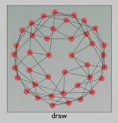
Executing all of that gets us something that's certainly promising:
Now we just need to make it pretty.
Exercise
- RelFinder let's you have more than two starting nodes (it does queries between all pairs). Refactor the list of queries to take a list of starting nodes.
Step 2d. Revising the drawing code
'''''Download the code for this step [springy4c.field.zip here].'''''
In fact, all that's missing now is some revisions to our drawing code. Most obvious of all, we're missing text labels for the nodes. Let's do that first, and let's only use the first few SPARQL queries to keep the graphs small while we iterate on them.
We need to add something to the geometry we are drawing for each node, so, we change makeMarker(...):
def makeMarker(node):
    m = FLine().moveTo(0,0)
    m.containsText=1 # ------ add some text
    m.text_v="   %s" % node.name
    m.rect(-w/2,-w/2,w,w)(derived#1, filled1, color=Vector4(0,0,0,0.5))
    m.eventHandler = SomeHandler(m)
    node.marker = m
    return m
Adding the attribute containsText tells Field's drawing system that this FLine can contain text; text_v is a vertex property that has a label on it. We're pulling out a name property of the graph node and display it. We need to make sure that getNode(...) puts that property in:
def getNode(m):
    n = nodeMap.get(m)
    if (n#None):
        global graph
        n # Cobj(urim, edges=[])
        n.name = m # ------ set the name
        nodeMap.put(m, n)
        graph += [n]
        kk.vertex.add(n)
    return n
The text label is conceptually part of the FLine, so we don't need to do anything else to ensure that it get dragged around with the existing mouse interaction we have setup for them. With these two additions we have:
Working! but those URI's are a little long winded:
def getNode(m):
    n = nodeMap.get(m)
    if (n#None):
        global graph
        n # Cobj(urim, edges=[])
        n.name = m.split("/")[-1].replace("_", " ") # --- better looking name
        nodeMap.put(m, n)
        graph += [n]
        kk.vertex.add(n)
    return n
Much better:
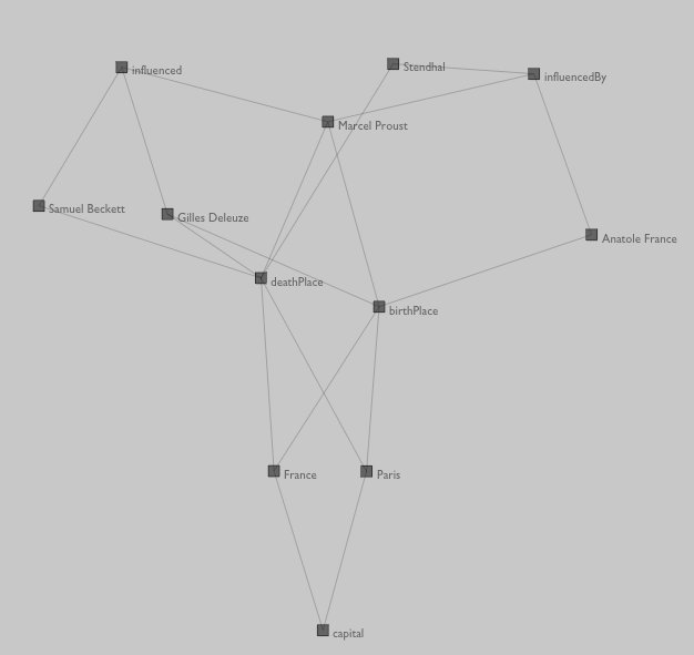
Of course, we are drawing directed edges (Object->Predicate->Subject) as straight lines. There's a big difference between Marcel Proust having influenced Samuel Beckett and Samuel Beckett influencing Marcel Proust. Let's replace our connection drawing code with this:
   c # FLine(derived1, color=Vector4(0,0,0,0.2))
    for n in graph:
        e = n.edges
        start = n.marker.events[0].position2()
        for m in range(len(e)):
            end = e[m].marker.events[0].position2()
            c.moveTo(*start)
            c.polarCubicTo(0.1,1,-0.1,1,end.x, end.y)

            along = (start-end).normalize()
            perp = Vector2(along.y, -along.x)

            cursor= c.cursor()
            cursor.setT(-0.6)
            mid = cursor.position()
            arrowSize=7
            c.moveTo(*mid-(perp-along)*arrowSize)
            c.lineTo(*mid)
            c.lineTo(*mid+(perp+along)*arrowSize)
The task is to draw the line between start and end with an arrow on a gentle arc. Highlights:
* .polarCubicTo(angle1,length1,angle2,length2, endPoint.x, endPoint.y) is a convenience function for drawing curves specified with respect to a straight line. Here we just want a little deviation from it.
* ursor= c.cursor() — Field's Cursor class helps analyze FLines. Here we're using it to find a point that's along the curve segment that we've just draw (back 0.6 or 60% from the end).
* .moveTo(*mid-(perp-along)*arrowSize) ... draws an arrow — it's just school math.
Note I wrote this code incrementally in about five attempts — off by a minus sign here, a change of mind about the size of the arrow there. When the time between testing .polarCubicTo(0.1... and .2 is under a second you can grow your code towards something that you find pleasing very quickly.
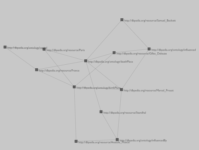
The result:
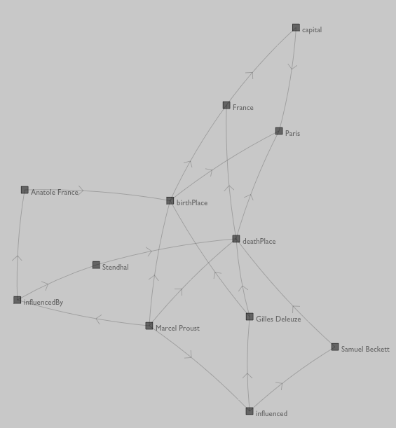
Getting there. But if you stare at this a little, you'll realize that we've made an interesting mistake. Unlike RelFinder, we've treated predicates on equal terms to subjects and objects — irthPlace has multiple edges entering and exiting it. Maybe this is interesting if you are interested in what kinds of objects cluster around predicates but it's pretty oddball otherwise — there's no way of telling from the graph above if France or Paris is the irthPlace of Proust and/or Deleuze.
The fault lies in makeConnection(...):
def makeConnection(o, p, s):
    p = getNode(p)
    o = getNode(o)
    s = getNode(s)
    if (not p in o.edges):
        o.edges.append(p)
    if (not s in p.edges):
        p.edges.append(s)
Let's change that such that predicates are unique given object and subject:
def makeConnection(o, p, s):
    p = getNode("%s %s %s" %(o, s, p))
    o = getNode(o)
    s = getNode(s)
    if (not p in o.edges):
        o.edges.append(p)
    if (not s in p.edges):
        p.edges.append(s)
This gives us the same graph as RelFinder — predicates are treated as uniquely defined by their context.
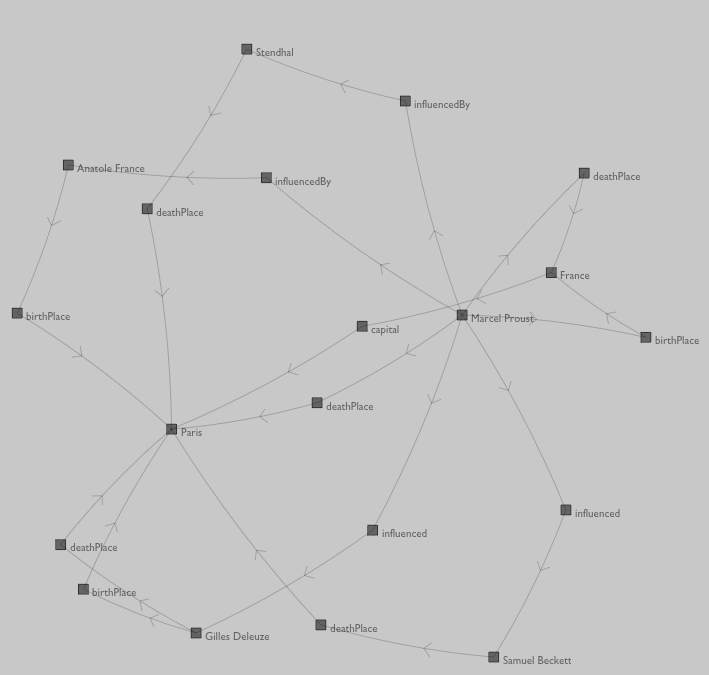
One final tweak to our drawing code: let's draw predicates differently to give them less visual clout.
def makeConnection(o, p, s):
    p = getNode("%s_%s_%s" %(o, s, p))
    p.ispredicate=1
... # same as before ...

def makeMarker(node):
    m = FLine().moveTo(0,0)
    m.containsText=1 # ------ add some text
    m.text_v="   %s" % node.name
    if (node.ispredicate):
        m.circle(w/4,0,0)(derived#1, filled0, color=Vector4(0,0,0,0.3))
    else:
        m.rect(-w/2,-w/2,w,w)(derived#1, filled1, color=Vector4(0,0,0,0.3))
.. # same as before ..
And since markers are created lazily there's no reason why we can't create two of them eagerly:
makeMarker(getNode(a)).color=Color4(1,0,0,0.5)
makeMarker(getNode(b)).color=Color4(1,0,0,0.5)
With a and b equal to "http://dbpedia.org/resource/Marcel_Proust" and "http://dbpedia.org/resource/Paris". Let's add a few longer SPARQL queries back in for the grand finale:
Exercises
I could keep tweaking this drawing code forever, but I'll stop. Fun things to try / think about:
- RelFinder makes quite a bit out of being able to highlight classes of object and predicate — following the last example, implement this kind of feature.
- RelFinder also let's you remove (and add back in) classes of object. You'll also have to remove all objects that become "unreachable" from your starting nodes. If you want to warm up to this, ''hiding'' is easier than ''removing''.
- Take a close look at these authorship examples. DBpedia seems to have been curated with a [http://en.wikipedia.org/wiki/The_Anxiety_of_Influence Bloomian] perspective — it's obsessed with influence. Find these influence predicates (there are a number that are used in a variety of situations
dbpedia.org/ontology/influencedBy,ontology/influenced,ontology/influences,property/influencedetc. These often encode the same relationship but with the arrow going the "other way". Try to normalize these relationships so that these diagrams only show influence — architecturally, where should this normalization occur? - Using Field's (ability to embed web-browsers directly)[EmbeddedWebBrowser] into the main UI canvas, include some version of RelFinder's web view panel.
Step 3a. Finishing up — Autocompletion for URI
We now have an unpolished, but certainly-polishable version of RelFinder's graph visualizer. I'd like take this excuse to two show two additional features of Field. RelFinder has a rather nifty auto-completing text boxes for entering the originating search terms. This is necessary because asking people to guess/type http://dbpedia.org/resource/Marcel_Proust rather than Marcel Proust is unreasonable. Can Field do something similar?
Here we go:
def dbresource(a):
    return "%s" % a

def completeFromDBPedia(m, text):
    qe = QueryExecutionFactory.sparqlService("http://dbpedia.org/sparql", """

SELECT DISTINCT ?s ?l
WHERE
{
?someobj ?p ?s .
?s <http://www.w3.org/2000/01/rdf-schema#label> ?l .
?l <bif:contains> "'%s'" .
}
LIMIT 20
    """ %text, "http://dbpedia.org")

    result = qe.execSelect()
    return ["%s"%n.get("?s") for n in result]

dbresource.__completions__ = completeFromDBPedia
This SPARQL query comes mostly out of RelFinder's network traffic (Jena has problems with the syntax of the one that RelFinder uses, so this one has been simplified a bit).
dbresource.__completions__ installs into the text editor "quotation" autocomplete (that's command-double-quote) for the function bresource. This means that if you hit command-" after bresource("Marcel you get:
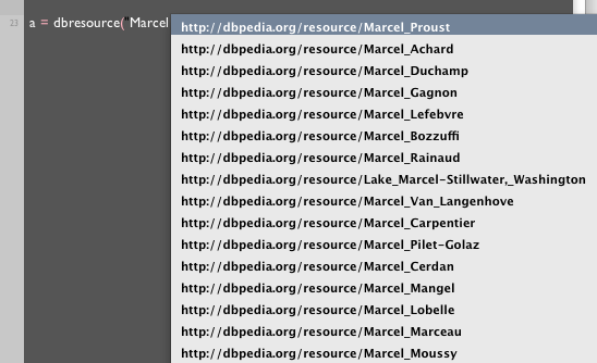
It acts just like command-period autocomplete — you can keep typing to refine the search. You could definitely imagine different kinds of SPARQL backed autocomplete.
Step 3b. Finishing up — Asynchrony
The second thing I'd like to touch upon briefly before we finish this "deep dive" into Field is support for multithreading. If you are playing with Field and RelFinder side by side you will have noticed two things — one, those SPARQL queries, especially the long ones, take time to complete — seconds, sometimes even 10 seconds or so. Secondly, RelFinder does an excellent job of burying this latency — slowly dripping the results of the first queries (that are basically instantaneous) onto the screen while the later ones are being processed. Field never has more than one query in flight at any time and worse submits them synchronously. Until they return, nothing, not even an animation frame, happens.
While this makes everything very easy to debug, it begins to wear a little thin after a while. There's a very straight-froward solution to this problem using a couple of new features of Field — SendToField and SendToExecutor:
In the heart of our SPARQL code we have something like:
def runQuery(q):
    result = q.execConstruct()
    processResults(result)

def processResults(result):
    for n in result.listStatements():
        print n
        o = n.getObject().toString()
        p = n.getPredicate().toString()
        s = n.getSubject().toString()
        makeConnection(o, p, s)
All we need to do is [http://www.python.org/dev/peps/pep-0318/ decorate] these functions to run them asynchronously.
from SimpleAsync import *

@SendToExecutor
def runQuery(q):
    result = q.execConstruct()
    processResults(result)

@SendToField
def processResults(result):
    for n in result.listStatements():
        print n
        o = n.getObject().toString()
        p = n.getPredicate().toString()
        s = n.getSubject().toString()
        makeConnection(o, p, s)
Instant multithreading! What's happening? the first decorator SendToExector causes all invocations of runQuery(...) to get sent to a pool of worker threads — the actual call itself appears to return instantly. The second decorator SendToField goes the other way — the work gets thrown into Field's main update loop (where previously all the work was getting done).
There are more flexible ways of doing multithreading, but none of them have fewer than two lines of code.
In fact, for two more, we can get even closer to our RelFinder model by moving the SendToField decoration to makeConnection:
from SimpleAsync import *

@SendToExecutor
def runQuery(q):
    result = q.execConstruct()
    processResults(result)

from java.lang import Thread
def processResults(result):
    for n in result.listStatements():
        print n
        o = n.getObject().toString()
        p = n.getPredicate().toString()
        s = n.getSubject().toString()
        makeConnection(o, p, s)
        Thread.sleep(1000) # --- pause for a 1000 milliseconds
]
@SendToField
def makeConnection(o, p, s):
    #.... as before ....
This will actually wait 1 second between adding the result of each query. Now we end up with something much closer to the rhythm of RelFinder.
Exercise
- Taking this last example make it interruptible — that is, devise a way to abandon all outstanding requests should you want to start again from the beginning (say, if the starting nodes change).
Conclusions
First of all the main result: we have what we set out to have — a working clone of the meat of RelFinder. It's largely unpolished, but it's fairly clear how we would proceed if we wanted to. '''Along the way we've written only: 6 Python functions, a small Python class that's a dozen lines long and hacked at a Java class that we found online'''. We have:
makeMarkerand the animation function that makes and draws geometry.getNodeandmakeConnectionthat make graph layout nodes and edges.processResultsandrunQuerythat actually send and interpret SPARQL queries.springUtilCobjis a recast part of the JUNG framework.dragHandleris our Python FLine interaction callback class.
From the outside it's impossible to make a fair comparison. But RelFinder appears to have over 100 individual source files and around 15,000 lines of code. How many of them are reused in other projects? I cannot say. Codebases this size, even when open-sourced and well documented, are difficult things to incorporate into this discourse of scholarship (for example, on my first reading I simply couldn't locate the SPARQL query generation code anywhere).
What we can say is that we've managed to do so much with so little because we've found in Field abstractions that are readily applicable to the problem of building things like RelFinder even though Field was never designed with this problem domain in mind. RelFinder's level of polish is impressive — it's as close to a "finished product" as we've ever seen in this area. But we've gotten so far so quickly because we've put aside, for the moment at least, any illusions of making a finished product; we've privileged research over development; we've deferred, perhaps indefinitely, the moment when documentation gets written, the boxes get closed up and everything gets given to "the client". There is no client. Rather, we've built a small environment for exploring something that ''we're'' interested in exploring, tailored specifically to the kinds of explorations we want to do — small, nimble, personal. With its source code, all 6 functions of it, sitting right there in plain view beckoning us.