Small examples
Coming to this site, you are almost certainly new to at least one of: Field, Python, Java, Computer Graphics or Programming. Most of the documentation on this site is about Field: its features, its ambitions, its relationships to other environments and libraries.
But this page is going to collect some very simple examples of Field in action. Just what you need if you are looking for something to get the ball rolling, a place to start.
First, a couple of important long pages for those coming over from the Processing environment. ConvertingAProcessingApplet is a long introduction to converting a Processing app into one that uses Field's Processing Plugin. If 2d drawing and printmaking is interesting, take a look at AProcessingTree, which converts a simple Processing exercise into Field's internal drawing system.
These pages are long and you should work through them (they'll tell you, for example, how to turn Field's Processing support on in the first place).
But some small concrete examples here should help cement that knowledge and enthusiasm.
Simple Processsing Event handling
A converted example from Daniel Shiffman's book "Learning Processing", courtesy of Timur Kuyanov
_self.a=0
background(0)
cursor()

def draw():
    stroke(255)
    strokeWeight(abs(p.mouseX-p.pmouseX))
    if _self.a:
        line(p.pmouseX ,p.pmouseY ,p.mouseX ,p.mouseY )

_r = draw

@p.onMousePress
def myMousePress():
    _self.a=1
    noCursor()

@p.onMouseRelease
def myMouseRelease():
    _self.a=0
    cursor()
This yields a very simple drawing program — put this code in a box and drag the mouse over the Processing window to draw a variable thickness line:
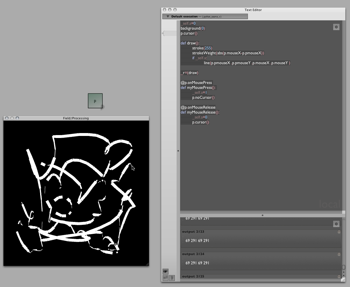
Note especially how Field handles the event handlers that this demo calls for. Since Field can have any number of boxes "running" all drawing things to the Processing window, Field lets you install, reinstall and uninstall event handlers using this special '@' syntax. Check out the longer tutorials for more examples.
A third party Processing Library — traer.physics
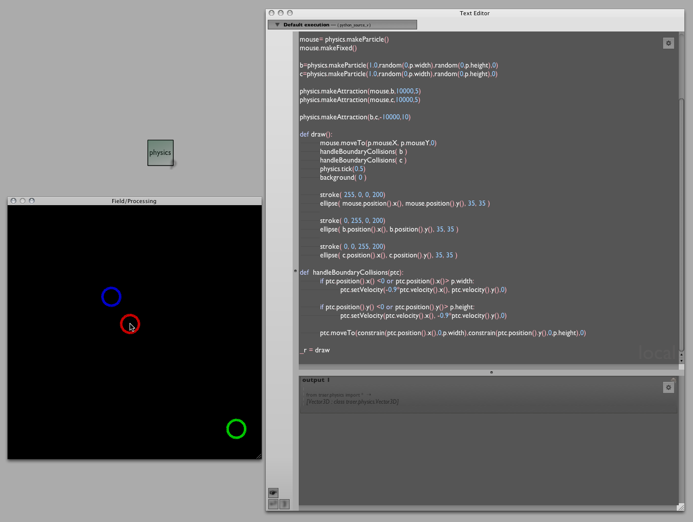
Traer.Physics is a popular simple particle system physics library for Processing. Well, that means it's a particle system physics library for Field as well. All you have to do is tell Field where you downloaded and unzipped the library to (using the Plugin Manager).
Here's one of their examples, converted for use in Field / Python, again courtesy of Timur Kuyanov:
from traer.physics import *

smooth()
ellipseMode(p.CENTER)
noFill()
strokeWeight(5)
noCursor()

physics= ParticleSystem(0,0.1)

mouse= physics.makeParticle()
mouse.makeFixed()

b=physics.makeParticle(1.0,random(0,p.width),random(0,p.height),0)
c=physics.makeParticle(1.0,random(0,p.width),random(0,p.height),0)

physics.makeAttraction(mouse,b,10000,5)
physics.makeAttraction(mouse,c,10000,5)

physics.makeAttraction(b,c,-10000,10)

def draw():
    mouse.position().set(p.mouseX, p.mouseY,0)
    handleBoundaryCollisions( b )
    handleBoundaryCollisions( c )
    physics.tick(0.5)
    background( 0 )

    stroke( 255, 0, 0, 200)
    ellipse( mouse.position().x(), mouse.position().y(), 35, 35 )

    stroke( 0, 255, 0, 200)
    ellipse( b.position().x(), b.position().y(), 35, 35 )

    stroke( 0, 0, 255, 200)
    ellipse( c.position().x(), c.position().y(), 35, 35 )

def  handleBoundaryCollisions(ptc):
     if ptc.position().x() <0 or ptc.position().x()> p.width:
          ptc.velocity().set(-0.9*ptc.velocity().x(), ptc.velocity().y(),0)

     if ptc.position().y() <0 or ptc.position().y()> p.height:
          ptc.velocity().set(ptc.velocity().x(), -0.9*ptc.velocity().y(),0)

     ptc.position().set(constrain(ptc.position().x(),0,p.width),constrain(ptc.position().y(),0,p.height),0)

_r = draw
This code, when stuck in a Field box and run, yields a little interactive physics demo. Mouse over the Processing window to drag the 'attractive' red circle around:
A Little computer vision — Hypermedia / OpenCV
OpenCV is the best thing that's happened to the Computer Vision community during it's existence; and there's a Processing library that exposes a little sliver of it. Follow the instructions here to get the library (and install the OpenCV framework) and tell Field where OpenCV.jar is.
Note: this library is exclusively a 32 bit library, which means that currently it does not work in 64 bit mode in Field.
We could just convert one of the examples straight from Processing — as usual, one sketch, one Field 'box' — but we can't resist making it a little more Field-ish. This example was provoked by Liubo Borissov, Assistant Professor at Pratt.
We'll use two boxes. The first contains some initialization code:
from hypermedia.video import *

opencv = OpenCV()
blobs = Blob()

val = 0
w,h = 320,240
threshold = 80

q = 0
opencv.capture(w,h)
opencv.read()
opencv.remember()

#Some versions of Processing have trouble resizing the canvas
#size(p.width, p.height, p.OPENGL,None)

def capture():
    opencv.read()

_r = capture
The second contains the actual demo:
def draw():
    background(0)

    opencv.convert( OpenCV.GRAY )
    opencv.blur(OpenCV.BLUR,4)
    opencv.threshold(128)
    opencv.flip(OpenCV.FLIP_HORIZONTAL)

    image(opencv.image(OpenCV.BUFFER),0,0,2*w,2*h)

    blobs = opencv.blobs(1000,w*h,4,False)

    noFill()
    stroke(255, 0, 0)

    if (len(blobs) > 0):
        for b in blobs:
            beginShape()
            [vertex(2*point.x, 2*point.y) for point in b.points]
            endShape(p.CLOSE)

_r = draw

@p.onKeyPressed
def keyPressed():
    opencv.remember()
Ran together these get us a cleaned up set of blobs (connected components). Blobs are just the kinds of things that you might be interested in tracking and tracked blobs form the basis of many an interactive piece (for example, multipoint frustrated total internal reflection interaction is basically an exercise in blob-tracking)
A screenshot:
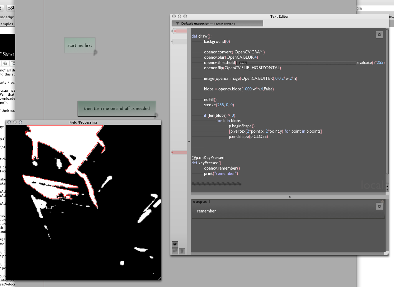
(You'll note that we couldn't resist replacing the magic constant '128' in the above code with a slider — setting that threshold is critical to getting the right number and kind of blobs).
Why the two boxes ?
In this example we transform what would have been a single file of a Processing Sketch into two Field boxes. Why? Well, the key thing is that we'd like to be able to experiment with code as fast as possible. While eliminating Processing 'stop-compile-go' cycle means that things are generally faster to play with in Field we can do better. This OpenCV library does a lot of work to set itself up properly — find the camera, start streaming information from the camera and so on. Ideally we'd do that once, and only once. So we move that work off to someplace else; it's own box. We start that, while we are writing the other box — the code that actually does something with the image. That code we write fairly live — line by line, looking at the contents of the OpenCV.BUFFER at each step along the way. Only at the end do we wrap that up in a function and make the box "runnable" with the variable _r. Even then starting and stopping this box is as simple as hitting command-PgUp and command-PgDown (or option-clicking on the box. This piece of code starts and stops instantaneously, the camera is constantly running.
Processing sound library — Minim
Minim is a brave attempt to clean up JavaSound into something that you'd consider using. It forms the backbone of Processing's simple sound support. Use in Field is straightfoward (example code from Liubo Borissov, Assistant Professor at Pratt.)
from ddf.minim import *
from ddf.minim.analysis import *
import math


m = Minim(p) # load minim class
w, h = 640,480
player = None
fft = None


def setup():
    #Some versions of Processing have trouble resizing the canvas
    #size(w,h,p.OPENGL,None)
    global player, fft
    player = m.loadFile(_self.dataFolder+"test.mp3",1024)
    player.play()
    player.loop()
    fft = FFT(player.bufferSize(), player.sampleRate())

def draw():
    background(0)
    n = player.mix.size()
    fplayer = []
    for i in range(0,n):
        fplayer.append( player.mix.get(i))

    # draw FFT
    fft.forward(fplayer)
    for i in range(0, fft.specSize()):
        x = map(i,0,fft.specSize(),0,w)
        stroke(255)
        #line(x,h,x,h-0.25*h*math.log(fft.getBand(i)+0.1,2))
        line(x,h,x,h-0.05*h*(fft.getBand(i)))

    #draw waveform
    for i in range(0, player.left.size()-1):
        x = map(i,0,player.left.size(), 0, w)
        stroke(100,100,255)
        line(x,0.25*h*(1+player.left.get(i)), x+1, 0.25*h*(1+player.left.get(i+1)))
        stroke(255,100,100)
        line(x,0.25*h*(1+player.right.get(i)), x+1, 0.25*h*(1+player.right.get(i+1)))

def stop():
    player.close()
    m.stop()

_r = (setup, draw,stop)
Gets you:
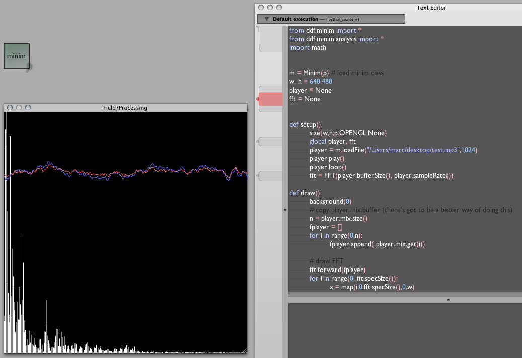
The only particularly Field thing to note is the use of _self.dataFolder to give us a path relative to the Field workspace. Otherwise it's as straightforward as conversions from Processing get.
ANAR+ — parametric modeling
ANAR+ is a very interesting Processing library for creating interesting pieces of geometry in Processing (note: creating interesting pieces of geometry is often called Architecture, Sculpture or Art).
Unlike Processing's immediate mode graphics system (but like Field's scene-graph graphics system), ANAR+ doesn't just draw geometry, but it keeps around the "construction history" of how that geometry is drawn.
In the case of ANAR+ this means that you can wiggle some of the original parameters went into your construction history and everything gets updated as if you redrew it all that way originally.
Such wiggling is just what Field is made for.
Here's a very simple conversion of a ANAR+ example into Field/Processing/Python. We are going to have two boxes, one that holds our initialization code and our very minimal draw function:
from anar import Anar, Pts, RenderPtsAll, Obj, Face

Anar.init(p)
Anar.drawAxis(1)
Pts.globalRender = RenderPtsAll()

form = Obj()

def draw():
    background(255)
    form.draw()

_r = draw
We'll start this one running and let it run forever. One more box will do the interesting stuff:
form = Obj()

bump = 10
moduleHeight = 50

for j in range(0, 1):
    a = [Anar.Pt(i*10, Math.sin(i/3.0)*bump, moduleHeight*j*2) for i in range(0, 80)]
    b = [Anar.Pt(i*10, Math.cos(i/3.0)*bump, moduleHeight*(j*2+1)) for i in range(0, 80)]

    for i in range(0, len(a)-1):
        myFace = Face()
        myFace.add(a[i])
        myFace.add(a[i+1])
        myFace.add(b[i+1])
        myFace.add(b[i])

        form.add(myFace)

    c = [Anar.Pt(i*10, Math.cos(i/3.0)*bump, moduleHeight*(j*2+1)) for i in range(0, 80)]
    d = [Anar.Pt(i*10, Math.sin(i/3.0)*bump, moduleHeight*(j*2+2)) for i in range(0, 80)]

    for i in range(0, len(c)-1):
        myFace = Face()
        myFace.add(c[i])
        myFace.add(c[i+1])
        myFace.add(d[i+1])
        myFace.add(d[i])

        form.add(myFace)

Anar.camTarget(form)
Our draw function just tells the top most Anar "form" — the top of their draw tree — to draw. Our principle box overwrites this form with something more interesting. So, as we are writing this box, we can continually jab (command-0 to execute all of the text in this box, and we'll immediately see the results on the screen.
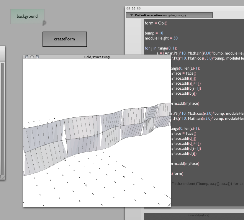
Because we haven't (just) drawn something, we've assembled a structure (form) that knows how to draw something we can hack our way back into it to modify it.
In another box, we can start playing with:
[aa.set(aa.x()+Math.random()*bump, aa.y(), aa.z()) for aa in flatten([a,b,c,d])]
After a few executions of that, we get:
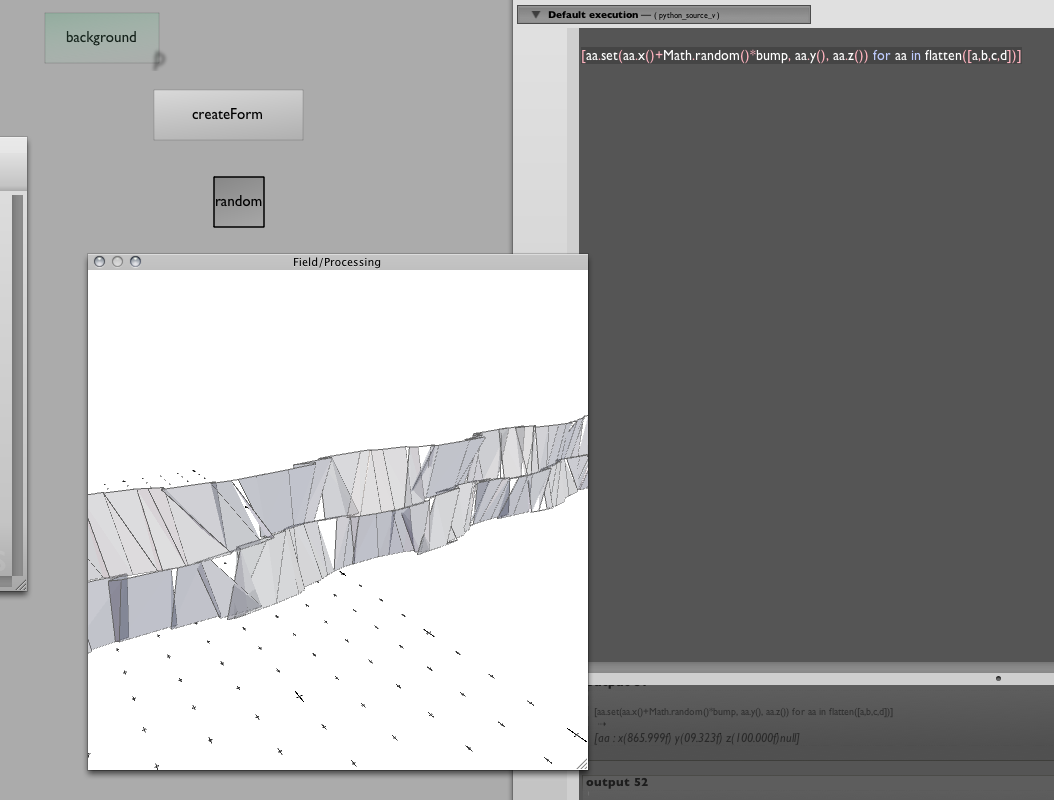
All in all it's a pretty interesting library — so interesting that I'd like to:
- rescue it from the confines of the Processing window and rendering model — to let it meet Field's FLine and 3d-FLine drawing model.
- provide some Python operator overloading magic to make using it's vectors, points, faces and so on more straightforward.
- integrate Field's sliders and other widgets with it's parameter model.
- Finally, integrate Field's Python tricks for late evaluation with ANAR+'s parameter model.
Work in progress.
Cheloniidae — turtle graphics done really well
People keep asking for something simple that they can noodle around with in Field to help them learn graphics, programming, Python or Field. Is there some simple, understandable library that, well, "does stuff" that they can play with? The truth is, I know what the answer is, I just haven't found the time to make it.
Well, now I don't need to. The answer, in general, is Turtle graphics. Turtle graphics is certainly what they used in my school to try and get the kids excited about computers (well, the kids who hadn't grown up hacking on a ZX81). It ought to be as fun today as it was then.
Well, it is — the Cheloniidae library by Spencer Tipping. I stumbled onto it and couldn't resist.
It's in Java and, as usual, a piece of cake to integrate into Field. Download it from http://projects.spencertipping.com/cheloniidae/ ,unpack it into some random directory in your downloads folder, tell the plugin manager about this folder (both as a folder of .class files and as a source folder).
I chose the pre-release version, because that's just the kind of person I am. This means some of the examples are out of date — no matter, Field's completion works just fine. Inspired by the example code, 5 mins later I have this:
from cheloniidae import *
from java.lang.Math import *

w = TurtleWindow()
w.setVisible(1)

t = StandardRotationalTurtle()
w.add(t)
t.lineColor(Color(0,0,0, 0.1))

def cube(size):
    for i in range(0, 4):
        square3(size)
        t.jump(size).turn(90)

def square3(size):
    for i in range(0, 3): t.move(size).pitch(90+Math.random()*1)
    t.jump(size).pitch(90)

for x in range(-4, 4):
    for y in floatRange(-2, 2, 10):
        for z in floatRange(-15, 15, 100):
            t.turn(0.59).pitch(0.6).position(Vector(x*100, y*100, z*100))
            cube(50)

w.setVisible(1)
Yielding:
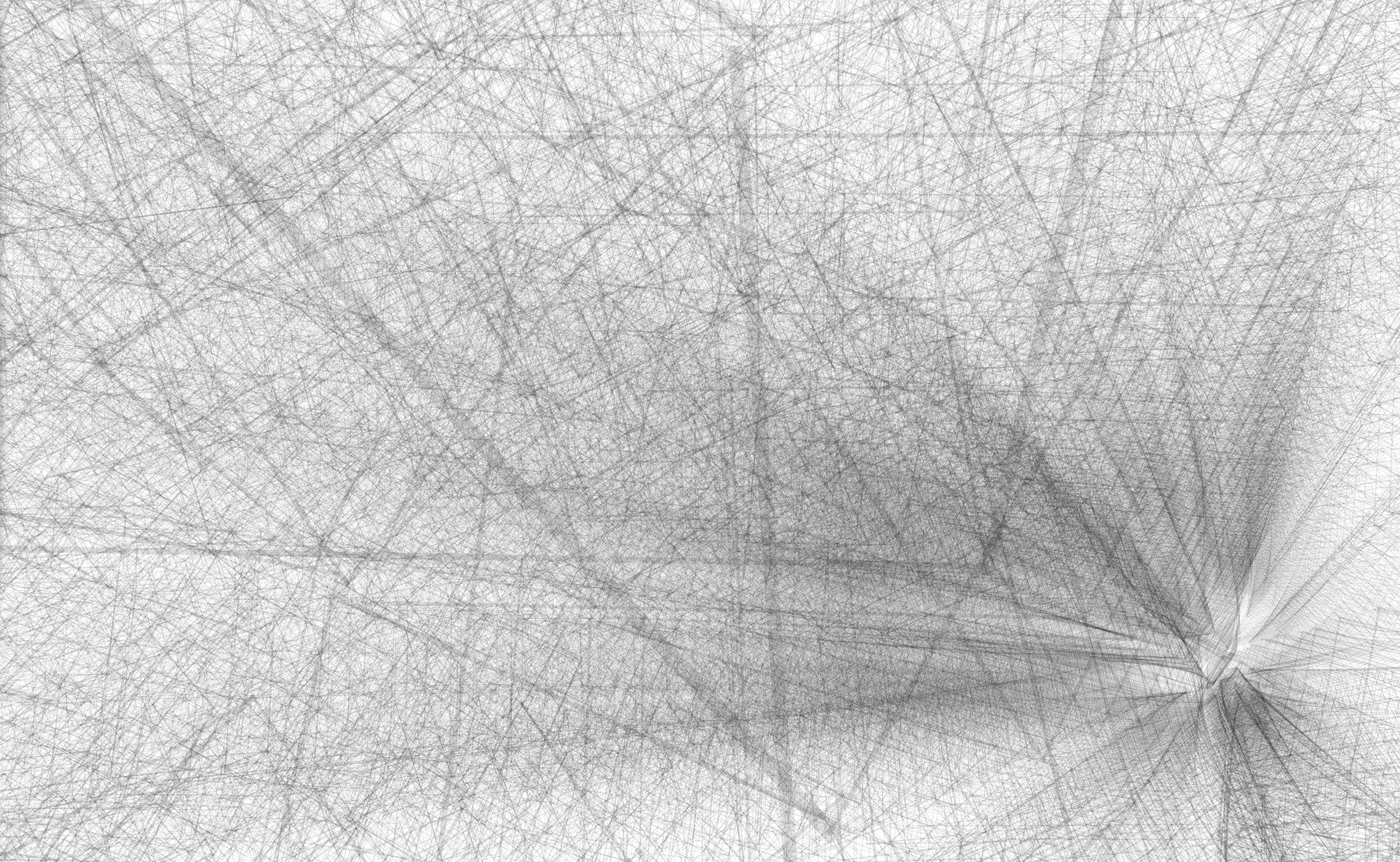 (click, as always, to enlarge)
How much fun is that? Actually more fun than it seems, because unlike Turtle graphics "back in the day", Cheloniidae stores the drawing in an intermediate form (a bit like Field's screen-graph graphics system). This means you get to rotate and zoom the camera for free. Now that's fun.
Sure, I'd prefer it if it emitted geometry to the FLine canvas drawing system or to the main graphics system. And, yes, I've no idea how to clear the drawing without closing and opening the window. But it's open source, so it may well do both these things soon.
I'm certainly going to have this library in my back pocket the next time somebody asks for something straightforward to play with.
Making a PDF (with Processing or Field)
How do I use Field to make a PDF? As usual, there are at least two answers. One is to use the PDF export functionality of Processing.
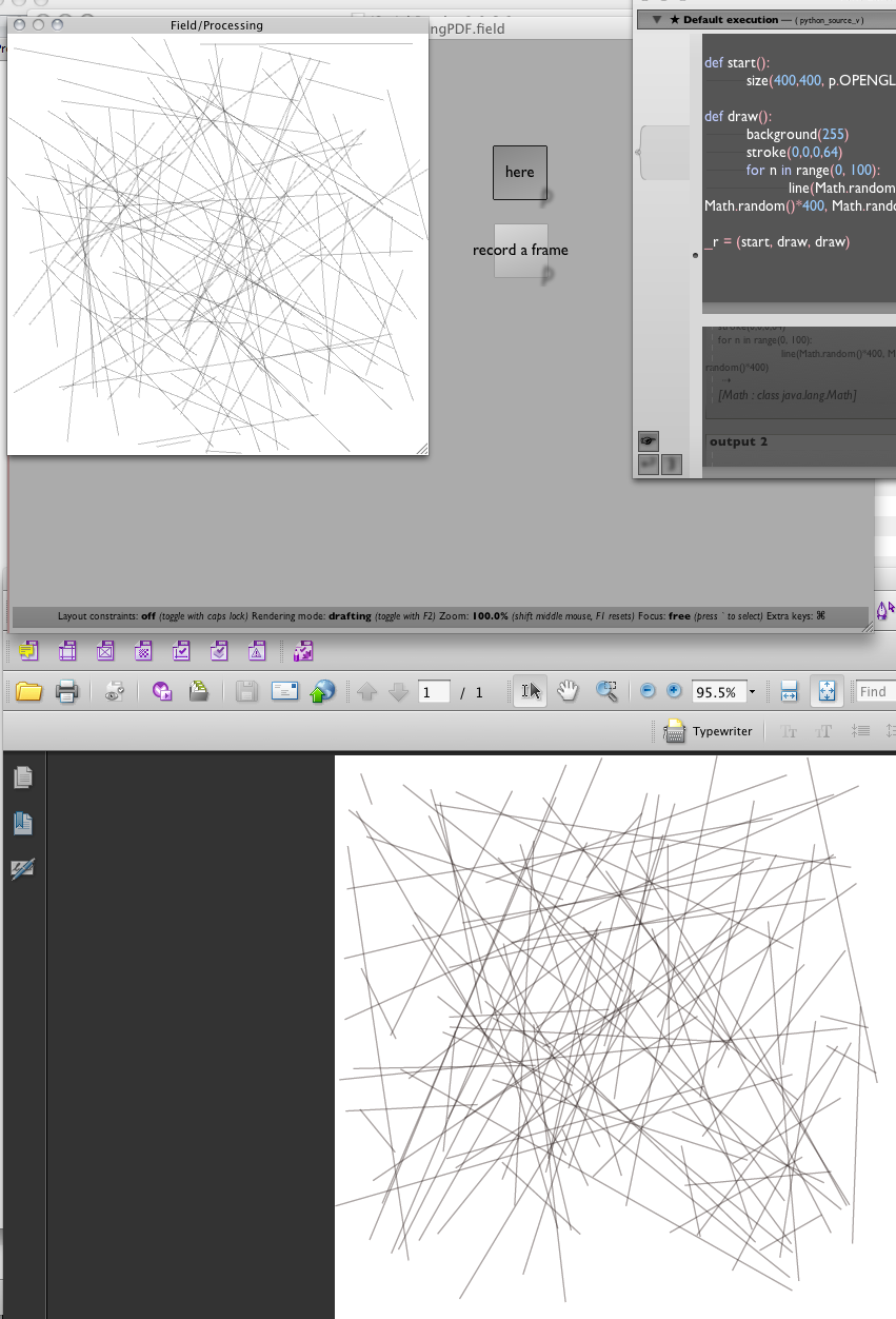
Let's I take a random example from http://processing.org/reference/libraries/pdf/index.html and convert it. In a new box we'll put:
def start():
    #this is optional if I like the default window size
    size(400,400, p.OPENGL, None)

def draw():
    background(255)
    stroke(0,0,0,64)
    for n in range(0, 100):
        line(Math.random()*400, Math.random()*400, Math.random()*400, Math.random()*400)

_r = (start, draw, draw)
As usually, I'll right click on this box and mark it as "bridged to Processing". I start this by option clicking on the box or apple-up'ing in the editor. Now I have an applet window with random lines animating in it.
Then elsewhere (say, in a different box) I can write and execute:
beginRecord(p.PDF, "something.pdf")
and later still
endRecord()
Between these two invocations I'll be making a PDF, and sure enough — I get a PDF with random lines in it:
While we're here, we note that we can skip Processing's draw cycle completely — after all, why animate if we are just trying to make a still? Executing this all by itself (in a box bridged to Processing) gives you a PDF:
beginRecord(p.PDF, "something3.pdf")
background(255)
stroke(0,0,0,64)
for n in range(0, 100):
    line(Math.random()*400, Math.random()*400, Math.random()*400, Math.random()*400)

endRecord()
FLine
That's the story for Processing/PDF/Field/Python. For Field itself you might want to take a close look at Field's own 2d / 3d-ish drawing system which is less about dynamic animation and more about static geometry. The documentation starts here — BasicDrawing — and continues through DrawingFLines, DrawingFLinesProperties, DrawingFLinesEditing, ThreeDFLines — and then gets to the bit that we're are interested in here ExportingPDFs.
In this case we can write:
_self.lines.clear()
for n in range(0, 10):
    p = FLine().moveTo(Math.random()*400, Math.random()*400)
    p.lineTo(Math.random()*400, Math.random()*400)
    p(color=Color4(0,0,0,0.25))

_self.lines.add(p)

makePDF(geometry=_self.lines, filename="/Users/marc/Desktop/aPdf.pdf")