Tutorial: Converting a Processing Applet to Field
Field's a different kind of beast than Processing's 'PDE' environment — different because there's more of it, different because it lets you write code in a different programming language (or four) but mainly different because it lets you write code inside the Processing Applet that you are creating while that applet is running. A shorter tutorial will hopefully have gotten you started using the ProcessingPlugin — the extension to Field that let's it talk to Processing Libraries, standard or otherwise. But some of that tutorial is duplicated here
This page is a narrative walkthrough of the process of converting a Processing Applet into Python and the Field/ProcessingPlugin (we also have a tutorial showing how to convert a 2d-Processing Applet into Field's PLine drawing system). Obviously converting applets from one environment to another isn't really the point of having an alternative Processing development environment and language (the point is to make new things in better ways). But in making such a conversion here we have an opportunity to highlight some of the differences (and some of the 'gotchas') between the two platforms and to express what we think is the potential of Processing on Field.
- The .field sheet that contains the code for this page can be downloaded here.
An example: SnakeDemo
Since OpenEnded hasn't and doesn't make any art using Processing, we turned to long-time friend and frequent collaborator Terry Pender (Associate Director, Computer Music Center, Columbia University) to see if he had something that fits on a page, but is complicated enough to throw up some useful issues and opportunities. He sent over a Processing applet called SnakeDemo. It's just what we needed, a rough, slightly messy, 'real-world' applet, fresh from the Sketchbook.
Getting started
First off, let's make sure that Field's bridge to Processing — the ProcessingPlugin — is actually turned on. In the Plugin manager we can determine the status of the Processing Plugin:
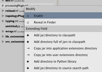
If you need to 'Toggle' processingPlugin.mf so that it becomes 'bold', and restart your Field environment. Field doesn't ship with Processing — we're not in the business of distributing it — you'll need a Processing installation from the usual sources and you'll need to stick it in the usual place (currently the Applications directory).
With the ProcessingPlugin on, Processing installed, and Field restarted, we'll now have a new tab on our inspector:
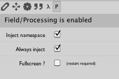
The exact contents of your window might be different. Go ahead and change the menu items to look exactly like the screenshot above.
Dependancies — third party Processing libraries
The SnakeDemo depends on one of those wonderful external, 3rd party Processing libraries, CellNoise, that Google tells me is available here http://carljohanrosen.com/processing/. Downloading the .zip file from that website gets you two things: a .jar file with the library in it (called CellNoise.jar) and a directory (called src) with the source code for the library. Field is interested in both of these things (although the latter is optional).
The simplest thing is you just drag this .jar file to the plugin manager and restart Field.
Optionally, we should also tell Field about the source directory (from the right-click menu), because Field can use the source code for a library to provide documentation and better auto-complete and inspection support for the classes contained therein. This puts important information about how to use the library at your fingertips while you are writing code and not off on a web-page somewhere.
With the .jar file and source path added (and Field restarted one more), we're nearly ready to begin.
A place to write code
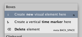
First, we'll need a 'new visual element' as a place to write our conversion to Field. On the canvas, right-click and select 'create new visual element' from the menu:
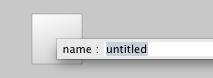
You'll need to give it a name in the text box that pops up:
When this element is selected, the text editor is now editing code that's 'in' this element. If you haven't already, you should go take a look at the documentation for the text editor.
One last thing. Because Processing makes special demands on when it's code is executed (for the technically inclined all Processing code is executing inside the applet's paint cycle), we need to tell Field that our newly created element is 'inside' the Applet:
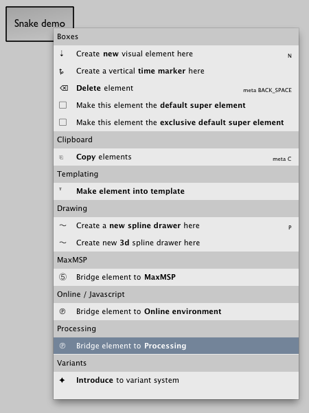
To remind us of this elements slightly special status, Field gives the element a badge:
Only code in such badged elements can draw things to the Processing Applet window.
Converting some Processing
And we're off! For reference purposes, we'll stick a copy of the original Processing/Java in a right hand side column ->
<div style="position: absolute; top:305em; left:600px; height: 500px; width:800px; border: 1px solid #ddd; padding-left:1em; padding-right:1em; background-color: #eee">
The original Processing/Java code
import CellNoise;

CellNoise cn;
CellDataStruct cd;
float[] freq = { 0.025, 0.025, 0.5 };
double[] at = { 0, 0, 0 };
float ax = 0, ay = 0, vx, vy;
float x, y, ox = 0, oy = 0;
float M, m, g, G, dt, t, odt = 0, h, w, strok, thick;

void setup() {
    size(1240, 800);
    background(255);
    cn = new CellNoise(this);
    cd = new CellDataStruct(this, 876, at, cn.CITYBLOCK);
    smooth();
    restart();
    M = 0.001;
    m = 500; // this affects the speed of the moving line
    G = 10;
    strok = 0.1;
    thick = 0.001;
}

void draw() {
    dt = (millis() - t) / 1000;
    if (dt >= 0.04) {
        t = millis();
        // println(x + ", " + y);
        at[0] = freq[0] * x;
        at[1] = freq[1] * y;

        cd.at = at;
        cn.noise(cd);

        // -----------------
        if (x > width + 10 || x < -10 || y > height + 10 || y < -10) {
            crash();
            restart();
            // mirror();
        } else {
            if (cd.F[0] < 0.1) {
                ax = M * m * G * (float) (cd.delta[1][0] / (cd.F[1] * cd.F[1] * cd.F[1]) + cd.delta[2][0] / (cd.F[2] * cd.F[2] * cd.F[2])) / freq[0];
                ay = M * m * G * (float) (cd.delta[1][1] / (cd.F[1] * cd.F[1] * cd.F[1]) + cd.delta[2][1] / (cd.F[2] * cd.F[2] * cd.F[2])) / freq[1];
            } else {
                ax = M * m * G * (float) (cd.delta[0][0] / (cd.F[0] * cd.F[0] * cd.F[0]) + cd.delta[1][0] / (cd.F[1] * cd.F[1] * cd.F[1]) + cd.delta[2][0] / (cd.F[2] * cd.F[2] * cd.F[2])) / freq[0];
                ay = M * m * G * (float) (cd.delta[0][1] / (cd.F[0] * cd.F[0] * cd.F[0]) + cd.delta[1][1] / (cd.F[1] * cd.F[1] * cd.F[1]) + cd.delta[2][1] / (cd.F[2] * cd.F[2] * cd.F[2])) / freq[1];
            }
            vx = (x - ox) / odt;
            vy = (y - oy) / odt;
            ox = x;
            oy = y;
            // println(dt);
            x = x + vx * dt + ax * dt * dt / 2;
            y = y + vy * dt + ay * dt * dt / 2;
            stroke(0, 255, 0, 56); // color of the ellipse
            ellipse(x, y, h, h); // the ellipse - the body
                        // of the snake

            h = h + w;
            if (h >= 200) {
                w = -0.75;
            } else if (h <= 0)
                w = 0.03;

            println(h);

            fill(random(237), random(159), 255, 90);// fill
                                // color
                                // for
                                // ellipse
            stroke(5, 5, 10); // this is the line inside the
                        // moving ellipse
            line(ox, oy, x, y);
            strokeWeight(strok);

            strok = strok + thick;
            if (strok >= 15) {
                thick = -0.1;
            } else if (strok <= 1)
                thick = 0.001;

            stroke(random(255), 0, random(117));
            ellipse(ox + (float) cd.delta[0][0] / freq[0], oy + (float) cd.delta[0][1] / freq[1], 3, 3); // these
                                                            // are
                                                            // the
                                                            // little
                                                            // randon
                                                            // dots
            ellipse(random(ox) + (float) cd.delta[1][0] / freq[0], oy + (float) cd.delta[1][1] / freq[1], 3, 3);
            ellipse(random(-oy) + (float) cd.delta[2][0] / freq[0], oy + (float) cd.delta[2][1] / freq[1], 3, 3);

            // stroke(5,9,255);
            // (sqrt(vx*vx + vy*vy) - 100);
            odt = dt;
        }

        // -----------------

        stroke(242, 04, 27, 45);
        line(x, y, x + (int) (cd.delta[0][0] / freq[0]), m + (int) (cd.delta[0][1] / freq[1])); // theses
                                                    // are
                                                    // the
                                                    // three
                                                    // lines
                                                    // that
                                                    // shoot
                                                    // out
                                                    // of
                                                    // the
                                                    // snake
        stroke(random(174), 221, 60, 45);
        line(x, y, x + (int) (cd.delta[1][0] / freq[0]), M + (int) (cd.delta[1][1] / freq[1]));
        stroke(15, 1, 255, 45);
        line(x, y, x + (int) (cd.delta[2][0] / freq[0]), g + (int) (cd.delta[2][1] / freq[1]));

    }
}

void restart() {
    float p = random(width * 2 + height * 2);
    if (p < width) {
        x = floor(p);
        y = -10;
        ox = x;
        oy = -11;
    } else if (p < width + height) {
        x = width + 10;
        y = floor(p - width);
        ox = x + 1;
        oy = y;
    } else if (p < width * 2 + height) {
        x = floor(width * 2 + height - p);
        y = height + 10;
        ox = x;
        oy = y + 1;
    } else {
        x = -10;
        y = floor(width * 2 + height * 2 - p);
        ox = -11;
        oy = y;
    }
    t = millis();
}

void mirror() {
    if (x < -10) {
        ox -= x;
        x = width + 10;
        ox += x;
    } else if (x > width + 10) {
        ox -= x;
        x = -10;
        ox += x;
    } else if (y < -10) {
        oy -= y;
        y = height + 10;
        oy += y;
    } else if (y > height + 10) {
        oy -= y;
        y = -10;
        oy += y;
    }
    t = millis();
}

void crash() {
}

void mouseReleased() {
    background(255);
    restart();
}
What we see there is a pretty standard, single file, piece of Processing code. Some imports (line 1), a bunch of declarations and initializations (lines 3-9), a setup method (11-23), a long draw method (25-119) and some helper methods at the bottom.
We are going to start at the top and work our way down. Here's where we're heading:
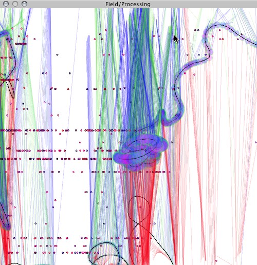
A point swoops around some smooth, endless, random curves, perturbed by the hidden cell noise structure while drawing lines out from the point in various directions. Simple.
Imports
Importing things in Field is easy. Line 1 says import CellNoise, in Python we're looking for something like:
from CellNoise import *
We could just write that and move on. Sometimes I forget to write the imports before I start coding — importing things is a drag — so the text editor offers some assistance. Start typing CellNoise and press command-i:
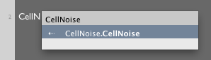
Since it's the only possible thing, you can just hit return (no mousing around required), and the import statement is added to the top of your text editor (and actually executed as well).
Declarations and initializations
Since Python is a dynamically typed language we're a lot less interested in declarations than we are initializations. Lines 3 and 4 have no equivalent in Python / Field. Lines 5-9 get a little shorter:
freq = (0.025, 0.025, 0.5)
at = (0.0, 0.0, 0.0)
ax, ay = 0, 0
ox,oy = 0, 0
odt, t, g, x, y, w, h = 1,0,0,0,0,0,0
M = 0.001
m = 500
G = 10
strok = 0.1
thick = 0.001
Arrays of floats and doubles in Processing become tuples. We've also taken the opportunity to move some of the variable initialization out of setup() back up here.
setup()
Lines 11-22 are almost straightforward. In Python/Field we'd start with:
def setup():
    background(255)
...
Field handles the setting of the Applet size, so it's best to omit that line. Next:
def setup():
    background(255)
    global cn
    cn = CellNoise(p)
...
Two things to note here. Firstly, global variables in Python are really the one place where the language introduces verbosity. Without the global cn declaration, the variable cn would never leave the setup() function. This is clearly not what we want. This is 'gotcha' number one (these will be summarized below at the end of this tutorial).
Secondly, while the original Applet's source refers to this (the Applet itself), the Applet in Field is the global variable p.
Continuing on:
def setup():
    background(255)
    global cn,cd
    cn = CellNoise(p)
    cd = CellDataStruct(p, 876, at, cn.CITYBLOCK)
    smooth()
    restart()
CellDataStruct is also in need of 'importing' and we can do that with command-i as we encounter it. The calls to smooth() (an internal Processing Applet call) and restart() (a helper method defined at the bottom of the source) complete setup()
So far, the Field/Python has paralleled the Processing/Java quite closely. But what we have is a little silly. In Field, there's no reason for any of this to be in some special method. Let's try this instead:
background(255)
cn = CellNoise(p)
cd = CellDataStruct(p, 876, at, cn.CITYBLOCK)
smooth()
And lose the setup() method altogether. Much better! For two reasons. Firstly, less typing is always better. Secondly, this style encourages us to execute code as we go along. By pressing command-return Field executes the current line or selection immediately. So we can check to see if background(255) is the color (white) that we want. We can check immediately to see if we've made any typos in cn = CellNoise(p) by executing it.
Having executed that line then we can then write cn. and press command-. (period) to 'see inside' cn, listing the methods and constants (and their documentation) that we could write after cn.. This is a much more interactive way of working, an it encourages a more experimental code practice. It's even a better way of coming to grips with somebody else's code. In the middle of a line of code, I have no idea what's in a CellNoise instance, and I can't be bothered to look at the source (or find the documentation). But I can be bothered to press command-. when needed:

If the library had more extensive JavaDoc-based documentation, it would appear there as well.
draw()
Having dismissed the setup() method into a few short lines of direct code, let's continue onward to the draw() method — the real meat of many a Processing Applet.
The first few lines are very straightforward:
def draw():
    dt = (millis() - t)/1000.0
    if (dt >= 0.04):
        t = millis()
...
But note, in passing, the explicit .0 at the end of 1000.0. In Python it pays to be explicit about division. While both Java and Python divide integers to get integers (3/4 # 0) in both languages, Java has explicit declarations of what's a float or not. Since we've sloppily declared t0 at the top, if millis() returns an integer then we'd probably be in a 3/4 = 0-like situation. In our case this means that dt will be 0 for a long time and then suddenly be 1, not the intention of the original author. This is the second 'gotcha' (see the list below).
Next, in line 30 and 31 we have, in the java:
at[0] = freq[0] * x;
at[1] = freq[1] * y;
What's going on here? Linear algebra is going on. Clearly at[0], at[1], freq[0], freq[1] and x and y are representing points or directions in space. Java has things classes like Point2d for storing the x and the y together in a single structure. But they aren't terribly useful. In Field/Python we can offer a little more support for doing simple things with points in space — see SimpleLinearAlgebra for more direct documentation.
Let's reorganize our code so far to actually express more directly these 2 dimensional quantities. All of the 'ox's and 'vy's and things become Vector2 instances. Like many a Java library these instances have methods for finding distances and computing angles and rotating things and so on. But in Python, you can also write a = b + c with Vector2s and have it do the right thing. This, and the clarity of having your 2 and 3 dimensional quantities actually expressed as such is worth taking a step back and doing properly. Taking it from the top, we now have:
from CellNoise import CellDataStruct
from CellNoise import CellNoise

freq = Vector2(0.025, 0.025)
at = [0,0,0]
a = Vector2()
o = Vector2()
position = Vector2()
odt, t, g, w, h = 1,0,0,0,0
M = 0.001
m = 500
G = 10
strok = 0.1
thick = 0.001

background(255)
cn = CellNoise(p)
cd = CellDataStruct(p, 876, at, cn.CITYBLOCK)
smooth()

def draw():
    global t,odt, h,w, strok, thick, position,o,a
    dt = (millis() - t)/1000.0
    if (dt >= 0.04):
        t = millis()
        at[0:2] = freq * position
        cd.at = at
        cn.noise(cd)

        delta = [Vector2(cd.delta[x][0], cd.delta[x][1]) for x in range(3)]

        if (position.x > width + 10 or position.x < -10 or position.y > height + 10 or position.y < -10):
            restart()
        else:
            if (cd.F[0] < 0.1):
                a = (delta[1]/cd.F[1]**3 + delta[2]/cd.F[2]**3)*M*m*G/freq
            else:
                a = (delta[0]/cd.F[0]**3 + delta[1]/cd.F[1]**3 + delta[2]/cd.F[2]**3)*M*m*G/freq

            v = (position-o)/odt
            position += v*dt + a*dt*dt/2
            o =position.clone()
...
There's not as much going on here as it looks (and there's much less of it than in the original Java, lines 1-58). Here are some of the highlights:
* at[tempting as it is, we can't actually changeatinto aVector2(or aVector3, it seems to have 3 elements) because it needs to be passed into the constructor ofCellDataStruct. Theat[0:2]=freq*position' notation sets the first two elements of the arrays at to whatever freq*position is.
* delta = [...] — we can radically simplify the code that follows by hoisting a lot of repeated code into this temp list. Note the compact use of a list comprehension to convert a useful Python data-structure out of a much more obscure pure-Java data-structure.
* **3 — Python has a convenient notation for exponentiation.
* v # (position-o)/odt — Here the use of Vector2 objects begins to pay off and we can compactly write exactly what it is that we're thinking about. Let's write it out in english: position continues (+) along the direction (v) it was traveling while accelerating along the direction a. It's either high-school physics or, if you prefer, almost exactly the text in wikipedia, symbol for symbol.
* o # position.clone() — o acts as the 'previous position'. It's not enough to write oposition because position itself is getting changed. What you want is a snapshot, a copy, a clone of position at this point in time.
The rest of the draw method is really the same story as this:
...
             stroke(0, 255, 0, 56)

            ellipse(position.x, position.y, h, h)

            h = h + w
            if (h >= 200):
                w = -0.75
            elif (h <= 0):
                w = 0.03

            fill(random(237), random(159), 255, 90)
            stroke(5, 5, 10)
            line(o.x,o.y, position.x, position.y)
            strokeWeight(strok)

            strok = strok + thick
            if (strok >= 15):
                thick = -0.1
            elif (strok <= 1):
                thick = 0.001

            stroke(random(255), 0, random(117))
            ellipse(o.x + (delta[0]/freq).x, o.y+(delta[0]/freq).y, 3, 3)
            ellipse(random(o.x) + (delta[1]/freq).x, o.y + (delta[1]/freq).y, 3, 3)
            ellipse(random(-o.y) + (delta[2]/freq).x, o.y + (delta[2]/freq).y, 3, 3)

            odt = dt

        stroke(242, 04, 27, 45)
        line(position.x,position.y, position.x+(delta[0]/freq).x, m+(delta[0]/freq).y)
        stroke(random(174), 221, 60, 45)
        line(position.x,position.y, position.x+(delta[1]/freq).x, M+(delta[1]/freq).y)
        stroke(15, 1, 255, 45)
        line(position.x,position.y, position.x+(delta[2]/freq).x, g+(delta[2]/freq).y)
restart()
Finally a helper method, restart().
width = p.width
height = p.height

def restart():
    global t, position, o
    xp = random(width*2 + height*2)
    if (xp < width):
        position = Vector2( floor(xp), -10)
        o= Vector2( floor(xp), -11);
    elif (xp < width+height):
        position = Vector2(width+10, floor(xp-width))
        o = Vector2(position.x+1, position.y)
    elif (xp < width*2+height):
        position = Vector2(width*2+height-xp, height+10)
        o = Vector2(position.x, position.y+1)
    else:
        position = Vector2(-10, width*2+height*2-xp)
        o = Vector2(-11, position.y)

    print "restarted %s " % (position)

    t = millis()
Note 'gotcha' number 3 — while we can write smooth() and ellipse() directly in Field, we have to access Applet fields through the Applet variable p. This is true for all variables that we traditionally can talk about directly in Processing. There's p.mouseX and so on. SimpleProcessingTutorial has more on this distinction.
Running it
For the purposes of completeness, I'll put the 'full' Python conversion on to the right hand side ->
<div style="position: absolute; top:855em; left:600px; height: 500px; width:800px; border: 1px solid #ddd; padding-left:1em; padding-right:1em; background-color: #eee">
The converted Field/Python code
<pre name="code" class="python">
from CellNoise import CellDataStruct
from CellNoise import CellNoise

freq = Vector2(0.025, 0.025)
at = [0,0,0]
a = Vector2()
o = Vector2()
position = Vector2()
odt, t, g, w, h = 1,0,0,0,0
M = 0.001
m = 500
G = 10
strok = 0.1
thick = 0.001

background(255)
cn = CellNoise(p)
cd = CellDataStruct(p, 876, at, cn.CITYBLOCK)
smooth()

def draw():
    global t,odt, h,w, strok, thick, position,o,a
    dt = (millis() - t)/1000.0
    if (dt >= 0.04):
        t = millis()
        at[0:2] = freq * position
        cd.at = at
        cn.noise(cd)

        delta = [Vector2(cd.delta[x][0], cd.delta[x][1]) for x in range(3)]

        if (position.x > width + 10 or position.x < -10 or position.y > height + 10 or position.y < -10):
            restart()
        else:
            if (cd.F[0] < 0.1):
                a = (delta[1]/cd.F[1]**3 + delta[2]/cd.F[2]**3)*M*m*G/freq
            else:
                a = (delta[0]/cd.F[0]**3 + delta[1]/cd.F[1]**3 + delta[2]/cd.F[2]**3)*M*m*G/freq

            v = (position-o)/odt
            o = position.clone()
            position += v*dt + a*dt*dt/2

            stroke(0, 255, 0, 56)

            ellipse(position.x, position.y, h, h)

            h = h + w
            if (h >= 200):
                w = -0.75
            elif (h <= 0):
                w = 0.03

            fill(random(237), random(159), 255, 90)
            stroke(5, 5, 10)
            line(o.x,o.y, position.x, position.y)
            strokeWeight(strok)

            strok = strok + thick
            if (strok >= 15):
                thick = -0.1
            elif (strok <= 1):
                thick = 0.001

            stroke(random(255), 0, random(117))
            ellipse(o.x + (delta[0]/freq).x, o.y+(delta[0]/freq).y, 3, 3)
            ellipse(random(o.x) + (delta[1]/freq).x, o.y + (delta[1]/freq).y, 3, 3)
            ellipse(random(-o.y) + (delta[2]/freq).x, o.y + (delta[2]/freq).y, 3, 3)

            odt = dt

        stroke(242, 04, 27, 45)
        line(position.x,position.y, position.x+(delta[0]/freq).x, m+(delta[0]/freq).y)
        stroke(random(174), 221, 60, 45)
        line(position.x,position.y, position.x+(delta[1]/freq).x, M+(delta[1]/freq).y)
        stroke(15, 1, 255, 45)
        line(position.x,position.y, position.x+(delta[2]/freq).x, g+(delta[2]/freq).y)

width = p.width
height = p.height

def restart():
    global t, position, o
    xp = random(width*2 + height*2)
    if (xp < width):
        position = Vector2( floor(xp), -10)
        o= Vector2( floor(xp), -11);
    elif (xp < width+height):
        position = Vector2(width+10, floor(xp-width))
        o = Vector2(position.x+1, position.y)
    elif (xp < width*2+height):
        position = Vector2(width*2+height-xp, height+10)
        o = Vector2(position.x, position.y+1)
    else:
        position = Vector2(-10, width*2+height*2-xp)
        o = Vector2(-11, position.y)

    print "restarted %s " % (position)

    t = millis()

</pre>
</div>
How to "run" this applet? Well, the Applet is actually already running — if you've been executing things like background(255) as you go along, you've been executing code 'in' the Applet all the time. If you like you can write draw() and then execute that (command-return), and you'll get a single frame of your animation. Really what you want to do is to have draw() called over-and-over (and note, unlike Processing, there's nothing special about the name draw(), it could be anything.
Field's approach to executing code (especially executing the same code over and over) is extremely polyvocal — see VisualElementLifecycles for a complete list. We'll use just one of the conventions for this, the special variable _r.
By adding:
_r = (restart, draw)
to the bottom of the code we tell Field that, to "run" this element over and over again, it should first call restart once and then call draw each 'animation cycle' . One of the ways to tell Field to go ahead and actually do that is to option-click on the element itself. It will turn green (to let you know that it's continuing to execute while you hold down the mouse and pop-up a menu that lets to tell Field to keep it running even when you release the mouse.
While the element is executing feel free to edit the original code — unless you take steps otherwise editing the code does nothing.
Of course, you can edit and execute additional code and that does something. For example, executing background(100) will clear the canvas to a mid-grey — so now you can make a slider on the canvas that changes the background color, live. The draw() will continue to run. Executing restart() will cause an immediate restart, so now you can make a button on the canvas that does just that (or just have a separate element that does that when option-clicked). Executing:
position[:]=(50,50)
o[:]=(51,50)
Will snap the position of the sweeping point back to (50,50) and send it off leftward.
You can have a completely different draw() method that does something else, in some other element, and start and stop that independently. You can put this element and others in timelines that you can scrub. And so on. SimpleProcessingTutorial has some more "Field"-ish ideas for where this idea might take you (also note language tricks like LazyFunctionalHelpers and GeneratorExamples). No compile cycle, no start and stop.
We think that changes everything about how things are made, but it also changes how made things are understood. If we take a look at the original Processing / Java — we'll see a few 'vestigial' pieces of code. Some commented out println statements and a whole uncalled method mirror(). In Field, you can print a global at any time — no need to stop, add a print call and then and then start again. This means that you can wait until something goes wrong (and perhaps stop the execution of your draw() functions) and then start printing out (or better) the contents of variables to find out what went wrong. Likewise, you can work on a mirror() function while the Applet it running and tune it's behavior by repeatedly running slightly different versions of it.
We also see something else that's very common — magic numbers. Line 4 and 10-4 have constants that govern the behavior of the Applet. "Tweaking" these things while the Applet is running is undeniably the best way of setting them in the first place. Bundling these numbers up into packages in ubiquitous in the digital arts — in animation this is a keyframe, in computer music this is a program, in lighting this is a cue — as is making sequences of these. Field can lead you quickly and with minimal code down these additional paths without you necessarily having to revise completely how you write code to make art.
Finally, we note that, just as Processing's development environment is acting as a 'gateway drug' for something more 'significant' like Eclipse or Netbeans, Field also encourages towards these more heavyweight, industrial tools. But with Processing's development environment the evolution from pure-PDE, then PDE+Eclipse, then pure-Eclipse has a very brief transition in the middle. Once you've conquered Eclipse and full syntax Java, the PDE doesn't have a tremendous amount to offer. Field tries to give you something that Eclipse doesn't, can't and won't and we spend our main development days with Eclipse and Field open side-by-side. Your own Java code-base is just as welcome in Field as Processing's is (almost all of the time Field can't tell the difference).
The Processing Plugin, and this tutorial, is designed to keep this intermediate, hybrid practice interesting for the Processing (library) artist.
Three 'gotchas'
During this conversion process we've noticed three things that people get caught on.
Global variables Python frowns on global variables where Processing smiles on them (they aren't really global, they are local to the Applet). In Python you have to declare the globals that you write to inside functions — it's one of the few places where Python adds syntax to slow you down. Well, careful, in Field, they really are global.
Processing Applet variables — Processing Applets have very important variables
width,heightandmouseX,mouseYand so on. Outside of the Processing Plugin these things basically don't exist or aren't relevant. Inside of the Processing Plugin these things are always referred to with explicit qualification asp.width,p.mouseXand so on, even if you have implicit qualification turned on (that is, your Processing Plugin tab says 'Always inject Applet into globals'). But watch for a handful of cases where a Processing method name (for examplemousePressed()shadows a Processing field name (here, the booleanmousePressed). In these cases we are trying to add accessors to these fields (in this case, anisMousePressed()method). Let us know what we've missed.Division — in both Java and Field
3/4actually equals0. Often you are expecting it to equal0.75. If that's what you were expecting, then you wrote it wrong. But sometimes the problem goes a little deeper in Python-based environments. While in Java you can writex/4and have somewhere elsefloat x # 3. If you "translate" that code into python you might write justx 3(Python doesn't need the 'float' part of that line). This gives you3/4again, very different from3.0/4. What you really mean is to writex = 3.0. This is so contentious in the Python community that they've promised to change it (indeed, you can change it throughout Field's Python environment by executing the magic incantation:from __future__ import division).
There's one more that, because of the kind of applet we've converted, we haven't noticed. But it's a popular gotcha nonetheless.
- Events — in Processing the names of methods are important:
draw()means draw andsetup()means setup. In Field you can call things whatever you like because you can have more than one of them. It's what you do with these functions thats important. What about event handlers likekeyPressed()andmouseClick()?. Field handles these things is special (and more powerful) ways. See the event hooks for more documentation.
Standard Disclaimer
Clearly we (the core developers of Field) think the Processing Plugin is great. (And we're most excited because the Processing Plugin code is actually only two short files long). But none of our previous or future commissions depend on it. This means we'll need the Processing communities support, bug-reports, code and ideas for it to flourish.