Field and Prosilica/AVT GigE cameras
Recently we've cleaned up and re-integrated "support" in Field for GigE vision cameras — specifically the ones supported by the Prosilica/AVT GigE SDK. We say "support" because, thanks to Prosilica's completely straightforward SDK all we're really doing is using Field to write code that makes calls into this SDK. We're using Field as a Java/Python hacking environment.
Still, we've built two things that might interest people — a couple of helper classes that link Prosilica's cameras to Field's graphics system (for preview or GPU based processing) and a small standalone utility that converts raw bayer files grabbed from the cameras to Adobe DNG files (for subsequent high quality de-mosiacing). Ultimately, it's always good to have more examples of Field "hosting" interesting code.
Getting started
As usual, first you need to tell Field where the SDK is. After downloading the SDK we build the project they supply in 'AVTGigESDK/Examples/Java/PvJPI' — this gets us the Java bindings to the SDK. Then, using the Plugin Manager in Field we tell Field that 'AVTGigESDK/Examples/Java/PvJPI/bin' contains a 'folder of class files'.
Next we need to add the .dylib's that are the native part of the SDK to Field. The easiest way of doing this it just to copy them into /Applications/Field.app/Contents/Resources/Java/ . Make sure you pick the x64 versions if you are using Field in 64-bit mode (the default).
Now we are in a position to write Python code that makes calls into the SDK. I'd make a new box and just check that this is the case:
from prosilica import *
print Pv.Initialize() #only call this once
Should print eSuccess.
At this point you should feel free to go read the SDK docs and do your own thing. (Remember CompletionAndInspection). All of the SDK lives, statically, inside Pv; none of it has Java-docs unfortunately.
Field Camera class
If you want to get something on the screen really quickly, tell the Plugin Manager about this jar. We'll be rolling this into the 'extras' folder of the development tree shortly. Now you gain access to a couple of helper classes that we've been using to capture and display raw sensor data off of the cameras. We're all about achieving the highest quality capture, so we limit ourselves to bayer16 (which is what we want to save to disk) and produce a de-mosaiced preview image on the GPU. If the words bayer and de-moasiced didn't mean anything to do, start reading. If you haven't read much about Field's graphics system expect you should.
To get an image on the screen we'll need a connection to the GigE camera and a place to render a texture map. Let's start with the camera connection:
from field.extras.gige import *
from prosilica import *

# this opens the first camera that it finds (automatically calls Pv.Initialize())
camera = Camera(".*")
camera.open()

# this class streams frames off of the camera and gives you a chance to process them:
streamer = StreamFrame(camera, 20)
To process the raw data from the camera, you'd write code like this:
frame = streamer.getFrameToProcess()
myBuffer = frame.ImageBuffer

#myBuffer is a java.nio.ByteBuffer that contains the raw bayer16 image data

# process.... process...

streamer.finishFrame(frame)
Communication with the camera is done asynchronously. Obviously, if you don't call streamer.getFrameToProcess() often enough, you'll start skipping frames.
Let's get that buffer on the screen using Field's graphics system.
from java.nio import ByteOrder
from java.nio import ByteBuffer

# a window to draw in
canvas = makeFullscreenCanvas()

# a shader to draw with
shader = makeShaderFromElement(_self)

canvas << shader

# a piece of geometry to draw
mesh = dynamicQuad_long()

shader << mesh

# our camera is 1280x960
w = 1280
h = 960

# this is a rectangle with the right aspect ratio
with mesh:
    mesh ** mesh ** [Vector3(0,0,0), Vector3(w/float(h),0,0), Vector3(w/float(h),1,0), Vector3(0,1,0)]

# these are texture coordinates
mesh.aux(_texture0, 2).put([0,0,w,0,w,h,0,h])
That gets us a plain dark grey quad in the graphics system — dark grey because we haven't customized the shader that's drawing it (nor have we added a texture to the shader).
Let's finish it. First the texture:
shader << streamer.createPreview(w,h)
This provides a rectangular texture that contains a floating point (luminance-only) version of the raw 16-bit bayer data. That is, there's no color information in this texture map.
While we've connected the texture map to the shader, we need to make the shader actually do some texturing. First let's just get it on the screen — the vertex shader:
varying vec4 vertexColor;
attribute vec4 s_Color;
attribute vec2 s_Texture;
varying vec2 texCoords;

void main()
{
    gl_Position = gl_ModelViewProjectionMatrix * gl_Vertex;
    vertexColor = s_Color;
    texCoords = s_Texture;
}
And the fragment shader:
varying vec4 vertexColor;
varying vec2 texCoords;

uniform sampler2DRect texture;

void main()
{
    gl_FragColor = texture2DRect(texture, texCoords);
    gl_FragColor.w = 1.0;
    gl_FragColor.xyz *= 16.0; // we're only using the bottom 12 bits
    gl_FragColor.xyz  = pow(gl_FragColor.xyz , vec3(1)); // you can change the gamma
}
This gets you something that looks like:
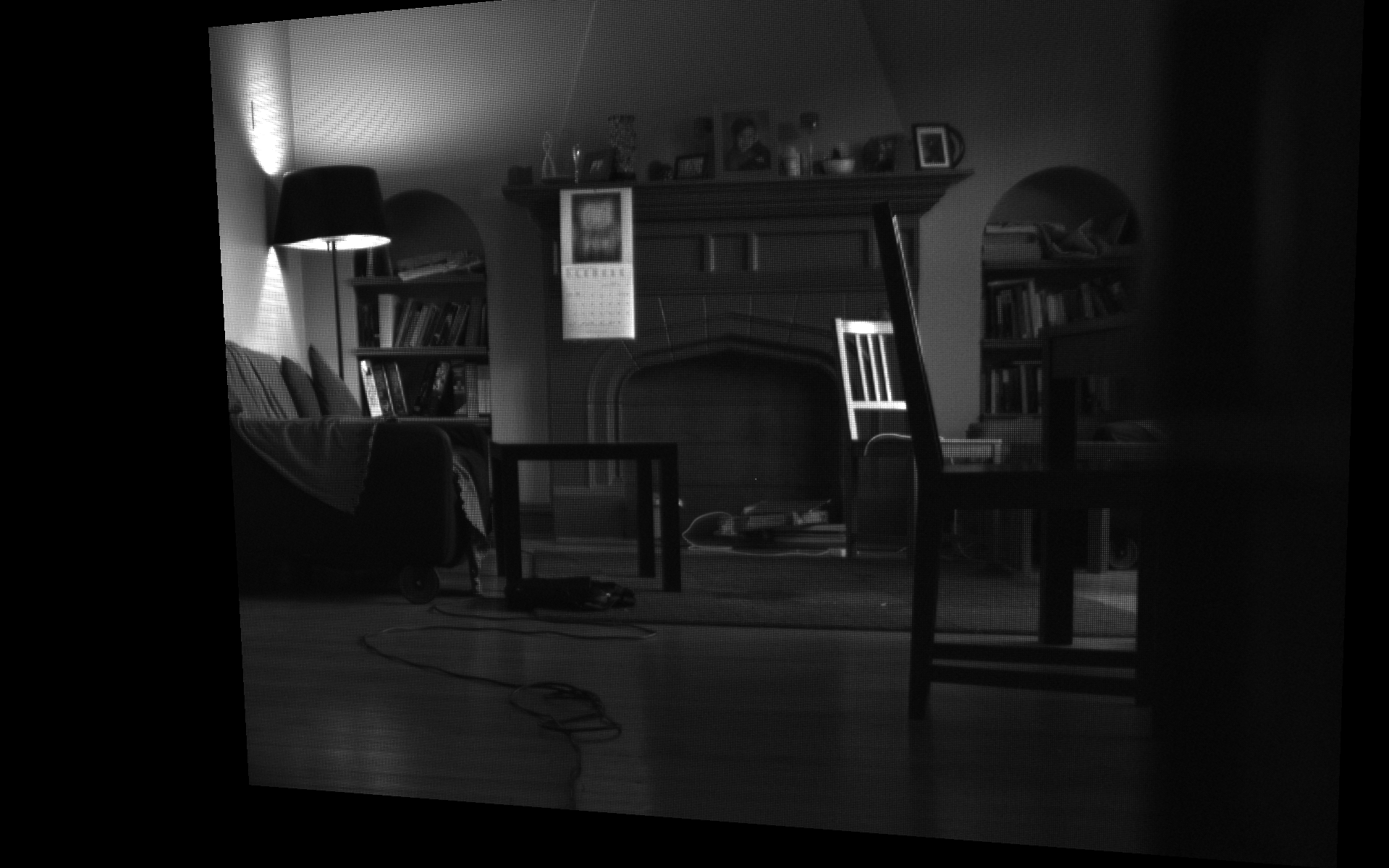
I've had to move the camera around using the keyboard — we're texturing a plane in 3d.
If you are using a monochrome camera, you can stop here, you're done. (Next you can try more interesting shaders, or processing the ByteBuffer directly).
In Color
If you are using a color camera, you'll notice some terrible moire patterns on this image. And, of course, you'll notice that it's not in color. Up close it looks like this:
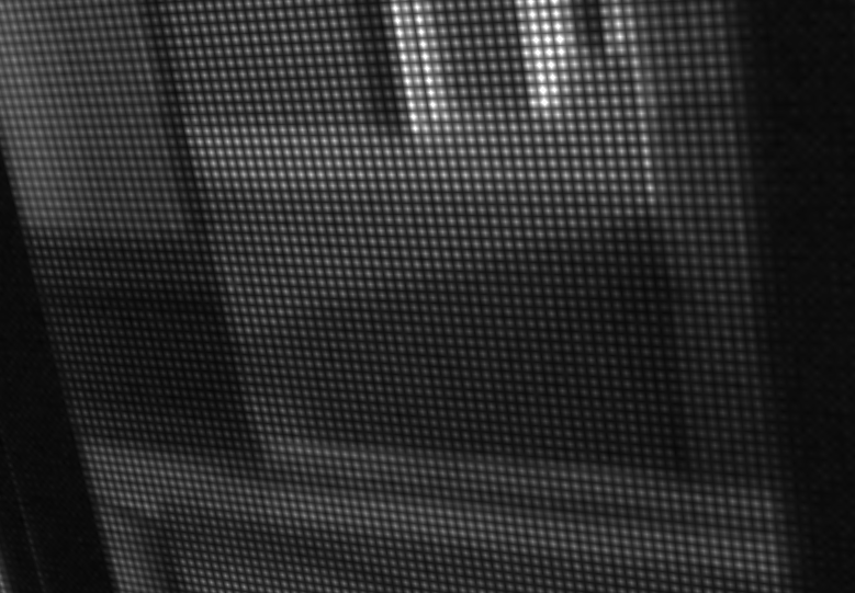
What you are seeing is the raw bayer pattern of your color camera. To actually see color, we need to de-mosaic this into a color image. Some Googling yields some very carefully written GLSLang GPU based de-moasicing code here. We'll adapt this to rectangular textures:
The vertex shader —
/** .xy = Pixel being sampled in the fragment shader on the range [0, 1]
   .zw = ...on the range [0, sourceSize], offset by firstRed */
varying vec4          centerR;

/** center.x + (-2/w, -1/w, 1/w, 2/w); These are the x-positions of the adjacent pixels.*/
varying vec4          xCoord;

/** center.y + (-2/h, -1/h, 1/h, 2/h); These are the y-positions of the adjacent pixels.*/
varying vec4          yCoord;

attribute vec2 s_Texture;

void main(void) {

    centerR.xy = s_Texture;
    centerR.zw = centerR.xy + vec2(0,0); // change this for different mosaics

    xCoord = centerR.x + vec4(-2.0, -1.0,1.0, 2.0 );
    yCoord = centerR.y + vec4(-2.0 , -1.0, 1.0, 2.0 );

    gl_Position = gl_ModelViewProjectionMatrix * gl_Vertex;
}
The fragment shader —
/** Monochrome RGBA or GL_LUMINANCE Bayer encoded texture.*/
uniform sampler2DRect          source;

varying vec4                      centerR;
varying vec4                      yCoord;
varying vec4                      xCoord;

void main(void) {

        #define fetch(x, y) texture2DRect(source, floor(vec2(x, y))+vec2(0.5)).r

        vec4 center;
        center.xy = centerR.xy; //floor(centerR.xy/2.0)*2.0;
        center.zw = center.xy+vec2(0,0);

        float C = texture2DRect(source, floor(center.xy)+vec2(0.5)).r; // ( 0, 0)
        const vec4 kC = vec4( 4.0, 6.0, 5.0, 5.0) / 8.0;

        // Determine which of four types of pixels we are on.
        vec2 alternate = mod(floor(center.zw), 2.0);

        vec4 Dvec = vec4(
                fetch(xCoord[1], yCoord[1]),    // (-1,-1)
                fetch(xCoord[1], yCoord[2]),    // (-1, 1)
                fetch(xCoord[2], yCoord[1]),    // ( 1,-1)
                fetch(xCoord[2], yCoord[2])); // ( 1, 1)

        vec4 PATTERN = (kC.xyz * C).xyzz;

        // Can also be a dot product with (1,1,1,1) on hardware where that is
        // specially optimized.
        // Equivalent to: D = Dvec[0] + Dvec[1] + Dvec[2] + Dvec[3];
        Dvec.xy += Dvec.zw;
        Dvec.x += Dvec.y;

        vec4 value = vec4(
                fetch(center.x, yCoord[0]),   // ( 0,-2)
                fetch(center.x, yCoord[1]),   // ( 0,-1)
                fetch(xCoord[0], center.y),   // (-1, 0)
                fetch(xCoord[1], center.y)); // (-2, 0)

        vec4 temp = vec4(
                fetch(center.x, yCoord[3]),   // ( 0, 2)
                fetch(center.x, yCoord[2]),   // ( 0, 1)
                fetch(xCoord[3], center.y),   // ( 2, 0)
                fetch(xCoord[2], center.y)); // ( 1, 0)

        // Even the simplest compilers should be able to constant-fold these to avoid the division.
        // Note that on scalar processors these constants force computation of some identical products twice.
        const vec4 kA = vec4(-1.0, -1.5,  0.5, -1.0) / 8.0;
        const vec4 kB = vec4( 2.0, 0.0, 0.0, 4.0) / 8.0;
        const vec4 kD = vec4( 0.0, 2.0, -1.0, -1.0) / 8.0;

        // Conserve constant registers and take advantage of free swizzle on load
        #define kE (kA.xywz)
        #define kF (kB.xywz)

        value += temp;

        // There are five filter patterns (identity, cross, checker,
        // theta, phi).    Precompute the terms from all of them and then
        // use swizzles to assign to color channels.
        //
        // Channel  Matches
        //  x           cross   (e.g., EE G)
        //  y           checker (e.g., EE B)
        //  z           theta   (e.g., EO R)
        //  w           phi         (e.g., EO R)

        #define A (value[0])
        #define B (value[1])
        #define D (Dvec.x)
        #define E (value[2])
        #define F (value[3])

        // Avoid zero elements. On a scalar processor this saves two MADDs and it has no
        // effect on a vector processor.
        PATTERN.yzw += (kD.yz * D).xyy;

        PATTERN += (kA.xyz * A).xyzx + (kE.xyw * E).xyxz;
        PATTERN.xw += kB.xw * B;
        PATTERN.xz += kF.xz * F;


        gl_FragColor.rgb = (alternate.y == 0.0) ?
                ((alternate.x == 0.0) ?
                        vec3(C, PATTERN.xy) :
                        vec3(PATTERN.z, C, PATTERN.w)) :
                ((alternate.x == 0.0) ?
                        vec3(PATTERN.w, C, PATTERN.z) :
                        vec3(PATTERN.yx, C));

    //gl_FragColor.rgb = texture2DRect(source, center.xy).rgb;
    gl_FragColor *= 16.0;

    gl_FragColor.w = 1.0;
}
Now we have a color image:
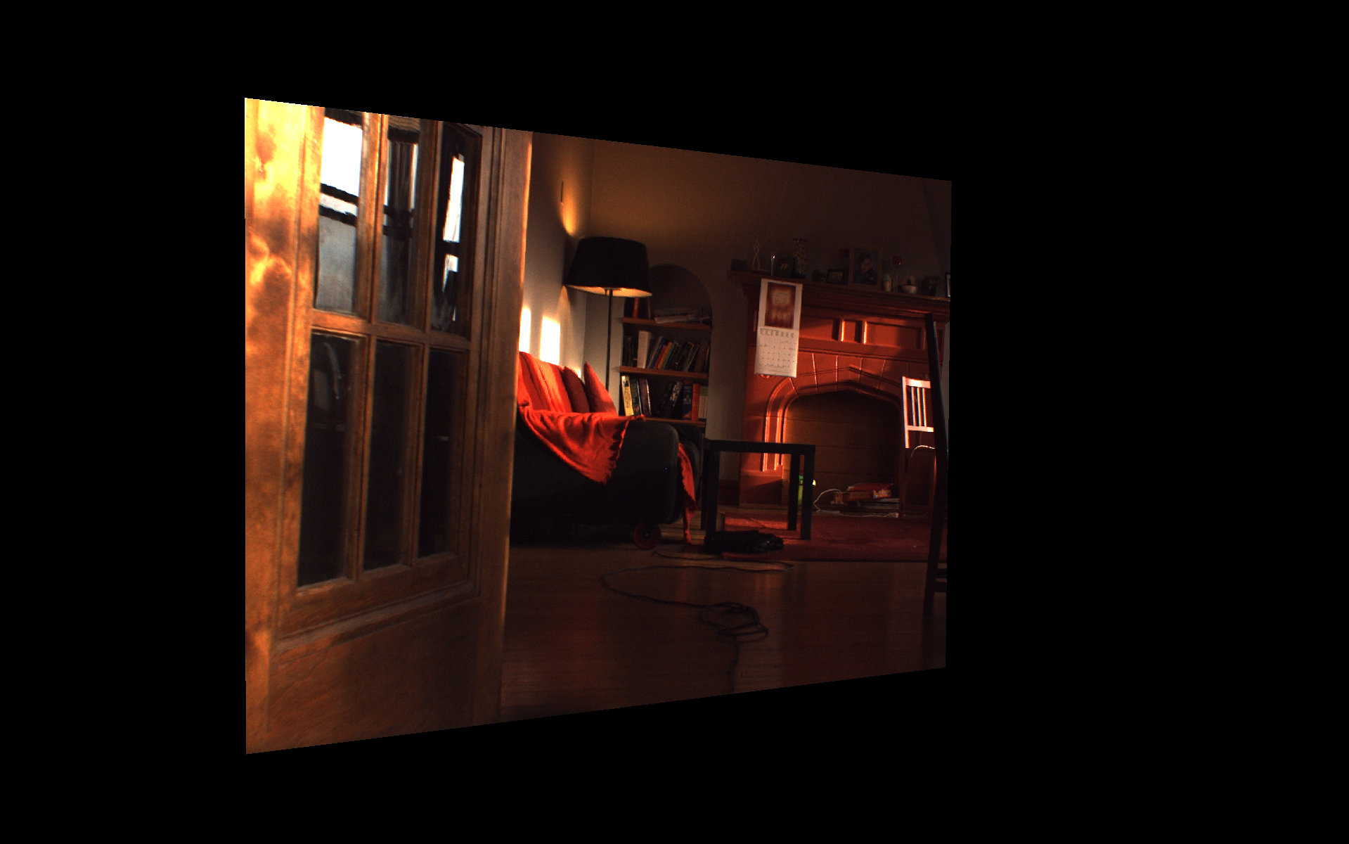
Obviously you are free to append any kind of GPU processing to the shader after the last line of the fragment shader.
Adobe Camera Raw
Over the next week or so we'll be turning this set of helper files into a full blown stereo raw capture system — we have two GC1290C cameras and we'll probably add a pair of GC690C's to the rig as well. One thing that we'd like to do is to capture raw sensor data and use a more heavyweight de-mosaicing system (the GPU based one above is good, but it's hardly state of the art and neither is the one built into the camera / API). Since we are "shooting raw" in the DSLR sense of the phrase it would be nice to be able to "develop" our video in the same was as you develop things from your stills camera. The trick then is to produce something that you can feed into a DSLR kind of pipeline.
Again, after much Googling around, we hacked together this utility — it takes "raw" 16 bit bayer files and adds just enough DNG to get things like Adobe Camera Raw (and Lightroom, Aperture and so on) to process the files.
As a convenience you can save these kinds of files out of Field:
f = streamer.getFrameToProcess()
f.ImageBuffer.rewind()
streamer.bayer16ToFile(f.ImageBuffer, "/var/tmp/firstBayer.bayer16")
streamer.finishFrame(f)
We'll be adding a much faster video format shortly.
Full usage and notes in the README file for the utility. In theory code like this ought to work for any source of raw bayer sensor data — the source code is short enough that you ought to be able to hack it pretty easily.