The Base Graphics System
Field is built on a OpenGL-based scenegraph library. It's ultimately how anything that appears in the canvas appears at all. Because Field is open source this means that Field comes with an OpenGL-based scene-graph library that you can use. And, because Field is a development environment, this means that you can use this library from within Field itself.
The library itself is wonderfully battle-tested (it has rendered most of the pieces on OpenEnded's main website).
We were rather hoping that during the year that Field has been kept under everyone's radars a 'competitor' scene-graph library that Field could publicly embrace would emerge. Since this hasn't really happened we feel there's room for a decent scene-graph library that's fairly fluid to use and yet captures contemporary OpenGL style.
Advanced real-time graphics in contemporary OpenGL style, unfortunately, can get a little advanced. If you are looking for a "traditional style" and pedagogically grounded way of putting triangles on the screen you will be much better served looking at Field's ProcessingPlugin. However, if you are looking to prototype some new GLSLang-based rendering techniques and need an graphics environment that's hosted in a "real" development language, Field might be just the thing for you.
If you are looking for more examples and documentation for using shaders in Field, don't miss BaseGraphicsSystem_Texturing.
Tutorial
Field's graphics system is covered in this downloadable tutorial.
Contemporary Style
What we're talking about with "Contemprary Style" OpenGL is the part of OpenGL that doesn't use any of the "fixed-function" graphics pipeline, opting instead to do everything that you can with shaders. In addition, "immediate mode" rendering while possible goes against the grain of this framework, and we opt instead for vertex buffer objects.
If the above paragraph (together with the links) didn't make any sense to you then this page is probably not for you. If it made at least some sense, then lets continue...
The AdvancedGraphics plugin
Shipping as an optional extension (you have to turn it on in the the plugin manager) is the AdvancedGraphics plugin. This doesn't actually contain the graphics system that we're describing — that's very much part of the core of Field (the package field.graphics.core to be precise). What it has is a small amount of Java and Python to make setting up networks of scene-graph objects very straightforward. Unlike the rest of Field and the underlying graphics system, this part is very much in flux, growing rapidly and under-tested. That's why it's an 'extra' for now. But we're developing it because there's an opportunity to make an extremely tight "pythonic" scene-graph library.
Hello Triangle
While in Processing (and hence Field) one appears to be able to draw a triangle using triangle(x1,y1,x2,y2,x3,y3), in the AdvancedGraphics plugin things are quite a bit longer winded and crucially conceptually different. We'll go through all the steps here in detail until we get to the end — we'll attempt to explain the benefits of this approach as we go.
First we need a place to draw our triangle:
canvas = getFullscreenCanvas()
This will return (and make if needs be) an open fullscreen canvas — either under Field's sheet, or, hopefully, on a second display. The background will be black (hence the lack of screenshot).
If you don't want to take over a display, you can write:
canvas = getWindowedCanvas(bounds=(30,50,100,200))
This opens a window at (30,50) that's 100x200 pixels big. Either way, we have a canvas now.
A shader
To draw anything in AdvancedGraphics we need at least two more things: some geometry and a shader to draw it. The shader is the program, written in a language called GLSLang, that runs on the graphics card. It takes geometry (and any addition information associated with that geometry) and some ad-hoc parameters and decides exactly how to turn that into pixels.
Crucially, we'll make for this triangular example, just one piece of geometry and one shader; and we'll attach them to the canvas just once. Having done this once our triangle will continue to draw itself without you writing any code to maintain it. If you are coming over from Processing's "immediate mode" graphics system this going to be quite a shift.
Here's one way of making a shader:
shader = makeShaderFromElement(_self)
This turns a code box into something that has a shader. How? It associates three new properties with element (in this case _self) and tells the text editor about them:
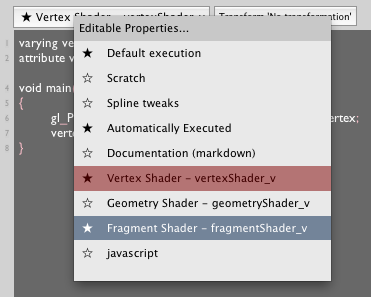
Secondly it fills in (if they haven't already been set) some sensible defaults for the vertex shader and the fragment shader (and leaves the geometry shader a sensible blank). At this point, you should go take a look at the OpenGL Shader language if you aren't familiar with it. That's the language that we're writing here.
Finally, makeShaderFromElement adds a button to the toolbar of the editor (when you have an element that's been turned into a shader selected) that recompiles the shader based on any changes you've made to it.
Some geometry
That's our shader sorted out — for now we'll just run with the default shader that makeShaderFromElement gives you. Now for a triangle:
mesh = meshContainer()
mesh is now an object that you can add two things to — vertices and triangles. These two things are related but clearly not the same thing.

One square, 4 vertices, two triangles — one triangle that goes 1,2,3 and one that goes 4,2,3.
So, to draw a triangle we need to add 3 vertices and one triangle to our mesh. In AdvancedGraphics we overload the operator ** to integrate both vertex and triangle data into meshes.
with mesh:
    mesh ** Vector3(0,0,0)
    mesh ** Vector3(1,0,0)
    mesh ** Vector3(0,1,0)
    mesh ** [0,1,2]
The first three ** operators concatenate three vertices (numbered 0, 1 & 2) into the mesh. The last line adds a triangle that spans these things.
We just happen to know that we've added vertex 0, 1 & 2. That's not always the case (if we were writing a library function 'append triangle' for example).
We can also do this:
with mesh:
    v1 = mesh ** Vector3(0,0,0)
    v2 = mesh ** Vector3(1,0,0)
    v3 = mesh ** Vector3(0,1,0)
    mesh ** [v1,v2,v3]
Great. But a little verbose. How about:
with mesh:
    v = mesh ** [ Vector3(0,0,0), Vector3(1,0,0), Vector3(0,1,0) ]
    mesh ** v
Or even just:
with mesh:
    mesh ** mesh ** [ Vector3(0,0,0), Vector3(1,0,0), Vector3(0,1,0) ]
You might be wondering what's with the with statement. If you are wondering what that even is it's new in Python 2.5. If you are wondering what it does, then we'll discuss it down below. For now let's just note that all drawing to mesh needs to be in (at least 1) with block.
Finally, if you are familiar with the FLine drawing system you can add FLines to containers:
mesh << FLine(filled=1).moveTo(0,0,0).lineTo(1,0,0).lineTo(1,1,0)
Note that in order to produce anything for a mesh the FLine has to be filled. As implied by the use of the << operator, the binding between mesh and any FLines attached to it is live — mutate the FLine and the mesh will be updated.
Shader + Geometry + Canvas = Hello Triangle
Now we are ready to put everything together. We need to attach shader to the canvas and the mesh to the shader:
canvas <<= shader
shader <<= mesh
AdvancedGraphics overloads the <<= operator to do 'attachment'. You can think of this as just making a hierarchy (actually what we are building has a little more structure than just a hierarchy, but you can usually get away with not thinking about this, see below).
And now, our triangle:
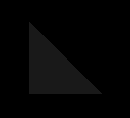 ]
]
It's so dim that, if you have a particularly miscalibrated monitor you might not be able to see it. But it's there — a triangle.
Editing the shader
It's dim because the default shader that we're using made it dim. Select the fragment shader in the text editor and you'll see this:
varying vec4 vertexColor;

void main()
{
        gl_FragColor = vertexColor+vec4(0.1, 0.1, 0.1, 0.1);
}
This fragment shader is adding a little bit of white to the (interpolated) vertex color. This is so when you draw something, as we have done, using the default shader and forget to add any vertex color information to the vertex you still see something. There's nothing worse than a blank screen in 3d graphics.
Checking the default vertex shader will confirm this:
varying vec4 vertexColor;
attribute vec4 color;

void main()
{
        gl_Position = gl_ModelViewProjectionMatrix * gl_Vertex;
        vertexColor = color;
}
Of course, if you just want the triangle red, you can edit the fragment shader:
varying vec4 vertexColor;

void main()
{
        gl_FragColor = vec4(1.0, 0.0, 0.0, 1.0);
}
And hit the refresh button on the toolbar.
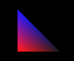
But how to associate color information with a vertex?
with mesh:
         v1 = mesh ** {_vertex : Vector3(0,0,0), _color : Vector4(1,0,0,1)}
         v2 = mesh ** {_vertex : Vector3(1,0,0), _color : Vector4(0,0,0,1)}
         v3 = mesh ** {_vertex : Vector3(0,1,0), _color : Vector4(0,0,1,1)}
         mesh ** [v1,v2,v3]
Gets us:
Under the hood
What's going on behind the scenes? "Traditional" Immediate-mode OpenGL is all about a large and diverse range of library commands — glTurnOnTheLightingType56 and glHereComesAVertex. These commands get executed over and over each frame of the drawing. In Processing's graphics system this is reflected in long draw() methods that do things. "Contemporary" OpenGL is about assembling a structure once, using very few library commands (and a flexible programming language), and then standing back while this structure (much of which is actually on the graphics card) just draws itself.
You can see a hint of this even in the trivial example above. You can pan and orbit around the full screen canvas with the keyboard (arrow keys walk around, shift-arrow keys orbit around). The canvas is clearly being updated, but a quick check of the Field sheet shows that nothing in Field is being executed.
It turns out that the mesh, and the shader are all "on" the graphics card. Of course there's some Java going on behind the scenes to remind the graphics card that it needs to draw that triangle with that shader, for each frame, but all that Java has been assembled ahead of time (with those << operators). But you will have to think about drawing 3d things differently. While it's more flexible than the "traditional" OpenGL, that flexibility is tied up inside, having to declare resources like shaders and meshes ahead of time is a different way of doing things. For scenes with more geometry that a triangle it turns out that this is vastly faster than immediate-mode OpenGL.
How much faster? Way faster. None of the computer games or applications that use OpenGL in a significant way draw in immediate mode. Likewise DirectX. It's so significantly faster to do things this way that the people in control of the evolution of OpenGL have been trying and failing to kill off immediate mode for a while now. It's conceivable that there will be a graphics card manufactured soon that will be unable to triangle() (without some pretty tricky software emulation). WebGL has no immediate mode of any kind; Google's o3d is an in-browser, in-JavaScript 3d graphics plugin and, guess what, it is a scenegraph library as well. In an odd way its things like Processing, and the pedagogical directness they embody, that's keeping the immediate mode in the drivers at all. Everybody else has moved on.
That with block
This difference — assembling a structure that knows how to draw itself vs. painting directly onto the screen — is the reason for those 'with' blocks you saw above. dynamicMesh (and dynamicLine and dynamicPoints) are willing to meet this fixed structure architecture and your code practice half way — you don't necessarily have to know up front how many triangles (lines or points) and vertices you are going to draw, and you don't necessarily have to promise not to change your mind. But you do have to tell the mesh when you're done drawing into it so that, if needs be, it can resize, reallocate, and refresh the geometry on the graphics card. Such a structure fits very will into Python's relatively recent with structure. Don't worry, they nest just fine.
What <<= actually does
You might also be wondering what kind of structure <<= assembles. The resulting structure is a lot like a hierarchy, but with ordered children. The goal is something approximating magic. While we wrote:
canvas <<= shader
shader <<= mesh
Above, we could also have written:
canvas <<= mesh
mesh <<= shader
Both ways, if you are thinking about it, make perfect sense. So, both ways work just fine. Once you have more than one mesh, you have to start making choices about how to assemble them:
canvas <<= mesh1
canvas <<= mesh2
mesh1 <<= shader
mesh2 <<= shader
Generally, it's better (shorter and slightly faster to draw) if the shared things go nearer the top, thus:
canvas <<= shader
shader <<= mesh1
shader <<= mesh2
We'll note in passing that you can also use <<
canvas << shader << mesh1 << mesh2
This helps compactly declarations:
shader = canvas << glslangShader("shaders/SimpleVertex.glslang", "shaders/AmbientFragment.glslang")
If we want to later "detach" these things from one another:
canvas | shader
shader | mesh
Think of | as a pipe that goes the wrong way. One word of warning: if you find yourself attaching and detaching things in the graphics system a lot (i.e. every frame of animation) you're probably thinking about the graphics system (and high performance OpenGL) wrongly. Graphics cards, and this graphics system, likes to set everything up once, then manipulate the contents of all of these shaders and meshes while animating.
More on shaders
Two things you'll need to know about shaders as soon as you start using them. First of all how to set uniforms — these are variables that are "global" to the program. The simplest way of doing this is directly:
shader.ambientColor = Color4(1,1,0,0.5)
will set a vec4 uniform variable called ambientColor to be that color.
Secondly, you'll want to know a little more about those per-vertex attributes.
In the example given above:
with mesh:
         v1 = mesh ** {_vertex : Vector3(0,0,0), _color : Vector4(1,0,0,1)}
         v2 = mesh ** {_vertex : Vector3(1,0,0), _color : Vector4(0,0,0,1)}
         v3 = mesh ** {_vertex : Vector3(0,1,0), _color : Vector4(0,0,1,1)}
         mesh ** [v1,v2,v3]
_vertex and _color are just synonyms for the integers 0 and 3.
In the default shader:
varying vec4 vertexColor;
attribute vec4 color;

void main()
{
        gl_Position = gl_ModelViewProjectionMatrix * gl_Vertex;
        vertexColor = color;
}
color is just helpfully bound to attribute 3 by Field. There's nothing special about the word color — that's the power and flexibility of shaders — you could rewrite this as:
with mesh:
         v1 = mesh ** {_vertex : Vector3(0,0,0), 5 : Vector4(1,0,0,1)}
         v2 = mesh ** {_vertex : Vector3(1,0,0), 5 : Vector4(0,0,0,1)}
         v3 = mesh ** {_vertex : Vector3(0,1,0), 5 : Vector4(0,0,1,1)}
         mesh ** [v1,v2,v3]
using an attribute numbered '5', and then picking this up in the shader:
varying vec4 vertexColor;
attribute vec4 s_Five;

void main()
{
        gl_Position = gl_ModelViewProjectionMatrix * gl_Vertex;
        vertexColor = s_Five;
}
Field declares s_One through s_Ten. There's more about this in LoadingFBXFiles#RawVertexdata.
Integration with PLine system
Now that we're finally beginning to expose Field's own graphics system one of the questions that we're asked a lot is, how can I draw a PLine inside this renderer? The surprising thing was, up until very recently, nobody inside OpenEnded had ever done such a thing. There was a real separation between the 'nice interface' PLine system and the 'speed and flexibility at all costs' main graphics renderer.
But, just recently, we had cause to write this code, and, as you'd expect, it's only really a few lines long. Thus you can write the following:
from CoreGraphics import *

canvas = getFullscreenCanvas()
_self.lines = canvas.lines()

_self.lines.clear()

line = PLine().moveTo(0,0).lineTo(10,10)(color=Color4(1,1,1,1))
_self.lines.add(line)

ii = image("file:///Developer/Examples/OpenGL/Cocoa/GLSLShowpiece/Textures/Abstract.jpg")
(ii<<blur(10)).show(decor=0)
This draws a line and draws a blurred image. If none the above code makes sense to you you should start with the PLine documentation — DrawingFLines for the geometry, CoreGraphicsExtensions for the image processing framework. Don't miss ThreeDPLines for information about how to make these lines actually 3d — otherwise you are drawing everything at z=0. Executing this you'll see the line and a soft blue glow. You'll quickly realize that you are staring at the inside corner of a (blured) image and a line from a very close distance. You'll need to move the virtual camera backwards to get a wider view.
The camera
Just how do you move the virtual camera? Two ways: with the keyboard (make sure you click on the canvas first); or with code.
Keyboard control
Using the keyboard, here are the keys you need: * the cursor keys rotate and translate the camera. Left/right rotate the camera and up/down moves it forward and back. This just like you were playing a first-person shooter (that is, as if they were 'WASD' rather than the cursor keys). * holding down shift holding down shift changes this 'walking around' behavior to be 'orbiting around'. Now left and right rotate around the center of interest (more of this below). * shift is sticky — releasing shift before you release the corresponding cursor key will let you keep orbiting without using the keyboard. * enter — on the numeric keypad stops all movement. * Page Up/Page Down rotate up/down, and as you might expect, if you are holding down shift, they orbit up and down instead. * 79 — on the numeric keypad "rolls" the camera (spins it clockwise or counter-clockwise along the direction of view). * finally 8246 — on the numeric keypad pans rather than rotates.
Code control
The keyboard is great for just taking a quick look at something you've made; but for careful and interesting work you clearly need some code control. The base class for a camera in Field's graphics system is BasicCamera and it's a real kitchen sink of camera control. We'll document just the essentials for now.
Field's camera really consists of 3 vectors (strictly speaking, two positions and a direction) — a position (where the camera is), a lookAt (what the camera is looking at) and an up direction (the direction of up). One thing you should note right off the bat — a camera that has a lookAt equals to its position (that is, it's looking at itself) or a up direction that lies along the direction between the position and the lookAt (that is, confuses 'up' with 'in') is a bad camera. Don't go there.
Setting the position, lookAt or up of a camera couldn't be easier:
#let's make a white triangle
canvas = getFullscreenCanvas()
shader = glslangShader("shaders/SimpleVertex.glslang", "shaders/AmbientFragment.glslang")
shader.ambient=Vector4(1,1,1,1)

mesh = dynamicMesh()
with mesh:
    mesh ** mesh ** [ Vector3(0,0,0), Vector3(1,0,0), Vector3(0,1,0) ]

canvas <<= shader
shader <<= mesh

#now lets set the camera
camera = canvas.camera
camera.position = Vector3(0,0,10)
camera.lookAt = Vector3(0,0,0)
camera.up = Vector3(0,1,0)
Because Field has nice support for Vectors and things, we can write things like this:
#move the position left
camera.position += Vector3(10,0,0)

#move the target up a little bit
camera.lookAt += Vector3(0,1,0)

#rotate the camera around the view direction a little
camera.up.rotateBy(Vector3(0,0,1), 0.5)
A few more numbers define a camera. fov is the field of view of the camera (which defaults to 45, and is inexplicably specified in degrees). Smaller numbers zoom the camera in; larger numbers zoom the camera out. A little more advanced is rshift and tshift translate the camera (left-right and top-bottom), producing an off-axis projection. It turns out that this is sometimes ideal for rendering in stereo and is the super-secret piece of math involved in tiling large displays.
Where next ?
Firstly, if you are interested in loading geometry and animation, you should next read LoadingFBXFiles. It's how complex pieces of geometry get loaded into Field; more on how traditional trees of transforms are done in Field and more on vertex data. After that there's BaseGraphicsSystem_Texturing — which has quite a bit more on texture, shaders, and the insides of the graphics system itself.
This page is just the early taste of exposing the 3d graphics system that Field uses to Field users itself. There are a great many other things already in the repository, most without carefully polished "Pythoninc" surfaces, but still ready to go. Everything you need to do very advanced graphics — Frame Buffer Objects, Geometry Shaders, Video textures, Skinning — as well as the things you'd probably expect in a graphics system — static textures and so on.
It's also fair to point out that while we feel that assembling scene-graphs with Python makes a great deal of sense, and prototyping things in Python likewise, drawing large or even medium amounts of dynamic geometry (geometry that changes every frame) using mesh ** Vector3() is slow and it's never going to get fast.
For that you really have one and a half options: 1) do what we do — and prototype and assemble scene-graphs (shaders, frame buffer objects and parameters to all of those) in Python and then manipulate the meshes as little as possible (pushing as much logic into the vertex and geometry shaders) and then always from Java. And option 1.5) use the embedded-JavaC support in Field to code small amounts of pure Java to populate those inner loops. The Java interface isn't as elegant as the Python one — it's in terms of java.nio.FloatBuffer and the like — but it sure is fast.