Drawing FLines; Some examples
Field let's you do all kinds of 2D drawing on its canvas using visual elements that contain drawing commands. On this page, we'll put the "reference" documentation for the central class that makes all of this possible — FLine — but for a more general overview see BasicDrawing.
Tutorial
The FLine drawing system is covered in this downloadable tutorial.
Reference
Reference material for creating geometry in here on this page; for changing the appearance of geometry see DrawingFLinesProperties and for editing and querying existing lines see DrawingFLinesEditing.
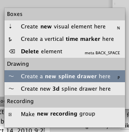
To run any of the examples in this page you'll need a visual element that's been configured to draw splines. Either make a new one (and then type in the name) using the menu, or pressing 'p':
or you take any old visual element and execute:
Mixins().mixInOverride(SplineComputingOverride, _self)
in it. This will "upgrade" the element to include the spline drawing helper properties.
What are the spline drawing helper properties? There's really only one: _self.lines is a list of things to draw: a list, that is, of FLine instances that contain the geometry that you'd like to put on the screen. There are some other helpful things that happen for boxes that draw splines, but _self.lines is by far the most important.
Getting started — .moveTo & .lineTo
Getting started:
_self.lines.clear()
myLine = FLine()
myLine.moveTo(75,75)
myLine.lineTo(100,100)
_self.lines.add(myLine)
This code does five things:
_self.lines.clear()— gets rid of any previous geometry associated with this boxmyLine = FLine()— makes a new, empty,FLineobjectmoveTo(75,75)— 'moves' this Pline's cursor to position 75,75lineTo(100,100)— makes a line from where the cursor is to 100,100_self.lines.add(myLine)— adds our line to the list of lines that need drawing
The coordinate system is such that 0,0 the origin is in the top left hand corner of the "page" with positive x going to the right and positive y going downwards. This is upside down from the typical cartesian presentation of coordinates but pretty typical in computer graphics (and is, in fact, the same order as this page is read in).
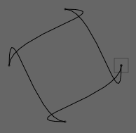
And thus, our visual element looks like:

The grey box is just the visual indication of the frame of this "box" (you can make that disappear/reappear completely by pressing f2 if you find it distracting). You get the box for free with the spline drawing functionality. The box moves around: it always tries to be near the lines that you put in it and it provides a stable place that you can always click on to select it (so that you can edit the code inside it). But, if you want to, you can also click on any spline that's part of this box's material.
Help for NodeBox and Processing users
Users coming over from NodeBox or Processing need to notice one additional thing about this first example. FLine is a Python class, so that myLine = FLine() makes a new instance of a FLine and assigns it to a variable called "myLine". All drawing gets done on and through these instances. While you are calling .moveTo and .lineTo and anything else you are not drawing on the screen, but rather you are simply adding instructions to your FLine object. At some point, you'll add this object to the list of things to be drawn, hence _self.lines.add(myLine) — if you don't, then you'll never see this line.
Both NodeBox and Processing often deliberately remove this apparent indirection for the sake of simplicity. For example, this code in NodeBox:
def curves(n=40):
    autoclosepath(False)
    beginpath(random(WIDTH), random(HEIGHT))
    for i in range(n):
        h1x = random(1000)
        h1y = random(1000)
        h2x = random(1000)
        h2y = random(1000)
        x = random(0, WIDTH)
        y = random(0, HEIGHT)
        curveto(h1x, h1y, h2x, h2y, x, y)

    return endpath(draw=False)
In this environment there's one line that you are drawing, and there's always one line. Once you are done with it you have to tell NodeBox not to put it on the screen. In Field you have to tell it to actually put the line on the screen. The equivalent code in Field:
#NodeBox has these set to be the dimensions of it's window. Field's canvas is infinite.
WIDTH=1000
HEIGHT=1000

def curves(n=40):
    path = FLine()
    for i in range(n):
        h1x = Math.random()*1000
        h1y = Math.random()*1000
        h2x = Math.random()*1000
        h2y = Math.random()*1000
        x = Math.random()*WIDTH
        y = Math.random()*HEIGHT
        path.cubicTo(h1x, h1y, h2x, h2y, x, y)
   return path
In NodeBox, you could then drawPath(curves()), in Field you would _self.lines.add(curves()).
What's the difference in the end? Well, two main things:
Field lets you work more naturally on a number of different lines simultaneously, while letting you pass these lines to (your own and anybody else's) functions even as they are still being drawn. This determines just how complex your drawing can get. For example if you want to temporarily hide a line in Field, just comment out the spot where it's added to
_self.lines. If you want to hide a line in NodeBox, you might end up having to track down where it getsendpath'd.If you are building your own libraries of drawing functions, who knows where that might be?Field encapsulates all of the things you can call (
cubicTo, moveToand so on) into one spot — theFLineclass. This gives you two benefits. Firstly, you can have other things calledcubicToandmoveTowithout clashing with the line drawing system; secondly it's easy to provide contextual help for the drawing functions: you just look at all the things you can do to and with aFLine. This is the basis for Field's in-place documentation system.
We think that these two benefits outweigh the extra typing and the cognitive overhead. We note that, should you really want to, you can always build a NodeBox/Processing style "state machine" style system out of the primitives given in Field. But it's exceedingly difficult to do in the opposite direction. And, finally, we get the impression (by squinting at the sources) that Processing itself is thinking about heading in this direction.
In the examples that follow, things like _self.lines.clear() and _self.lines.add(someLine) have been left off. So you'll have to pay a little more attention.
Chaining things together
It's worth noting that FLine methods that don't have anything better to return, return the FLine itself. This means that we could write our original example in a single line:
myLine.moveTo(75,75).lineTo(100,100)
A line is a sequence of such segments, and the "cursor" moves to where this line now is. This means that we can write:
myLine.moveTo(75,75)
myLine.lineTo(100,100)
myLine.lineTo(150, 100)
myLine.moveTo(90,85)
myLine.lineTo(105, 85)
Which gets us this:
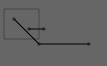
Note the connected line segments (two .lineTo in a row) and the skip (the second .moveTo).
Essentially what happens is this: the pen goes down, draws a line segment, draws another line segment, then picks up the pen, moves it, and draws another line.
Shorthand
Finally we note that typing out moveTo and lineTo can get very tedious fast. Field allows you to compress them to m and l, giving you things like myLine.m(75,75).l(100,100). (And you can get the abbreviations possible at any time with autocomplete.) We'll keep the long form in example code here for readability.
Curves: .cubicTo
So much for straight lines. Field handles curved segments as well:
myLine.moveTo(75,75)
myLine.cubicTo(100, 75, 75, 100, 100, 100)
produces:

cubicTo(cx1, cy1, cx2, cy2, x2, y2) produces a curved segment (a "cubic spline") that goes from wherever the FLine cursor is to x2, y2 using cx1, cy1 and cx2, cy2 as intermediate control points.
By selecting the points in Field we can cause it to draw these control points:

You ought to be able to convince yourself that these hidden intermediate points are in fact at 100, 75 and 75, 100 respectively. The line doesn't go through these points, it just inflects towards them along the tangents described by these control points.
Just as .moveTo and .lineTo have compressed synonyms m and l, .cubicTo can be written as .c.
Other ways of making curves: .relCubicTo & .polarCubicTo
.cubicTo should be pretty obvious, but it can be inconvenient. Sometimes you want to draw a line that is straight-ish but bends a little in some direction or the other. Using .cubicTo you have to remember where the FLine's cursor is and do some math to make the correct control points. .relCubicTo does this for you:
myLine.moveTo(75,75)
myLine.relCubicTo(20, 0, -20, 0, 100, 100)
relCubicTo(dx1, dy1, dx2, dy2, x2, y2) makes the control points by displacing points that trisect the straight line from the cursor to x2, y2:

In the picture above, the part of the line close to the start has been nudged right by 20 units (hence 20,0) and the part near the end has been nudged left by 20 units (hence -20, 0).
.polarCubicTo is similar and helpful in similar situations:
myLine.moveTo(75,75)
myLine.polarCubicTo(-1, 1, -1, 1, 100, 100)

polarCubicTo(angle1, length1, angle2, length2, x2,y2) again displaces the midpoints of the line between the cursor and x2,y2. In this case, it rotates the mid-point around the start (angle1) or the end (angle2) of the line and then scales it by length1 or length2 respectively.
A quiz to check your understanding: you should be able to work out why both polarCubicTo(0,1,0,1, 100, 100) and polarCubicTo(1,0,1,0, 100, 100) give you a straight line.
(Answer: in the first case, the midpoints aren't rotated at all and are scaled by '1'— i.e. just left the same; in the second case the they are rotated, but then they are scaled by '0' — i.e. reduced to being just the start and end points themselves).
.circleTo
Finally, one more way of making curves. Rather than specifying a destination and some control points that 'inflect' the curve towards them but don't actually pass through them .circleTo(x1, y1, x2, y2) uses part of the circle that is uniquely defined by the cursor and the next two points x1,y1 and x2, y2.
circleLine = FLine().moveTo(60,60).circleTo(56, 95, 80, 100).circleTo(70,70, 60,60)
yields:

(Note that circular arcs are decomposed into a small number of cubic splines, so if you are looking at Field's guide 'dots' that it draws for selected visual elements you might see a few more then you expect).
.position field
The methods above help you avoid a little math in the most common cases. But sometimes you need to know the position of the cursor: .position returns the current cursor position of the line:
somePlace = myLine.position
It returns a Vector2 object which (as you can tell from autocompletion) has all kinds of useful things for doing 2D geometry. There's much more information on the useful Vector2 class (and its higher dimensional friends, Vector3, VectorN and Quaternion) here.
Premade shapes: .rect, .circle, .ellipse, .appendShape
Everything so far has been assembling lines with the very simplest atoms: straight lines and simple curves. How about something a little more convenient?
.rect(r) — appends a free standing Rect to the FLine. A Rect is Field's data-structure for holding a Rectangle. Therefore, FLine().rect(Rect(50,50,20,30)) is a line with a rectangle in it, the top-left corner is at 50,50 and it's 20 wide and 30 long.
.circle(radius, x, y) — appends a circle centered on x,y and .ellipse(radius_x, radius_y, x, y appends an ellipse.
.line(x1, y1, x2, y2 — is simply a shorthand for .moveTo(x1, y1).lineTo(x2,y2).
Copying, Translating, Rotating and Scaling
The code above concerns making geometry, often line-segment by line-segment. Another way of making geometry is by filtering, transforming, or editing some other piece of geometry.
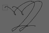
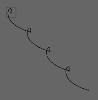
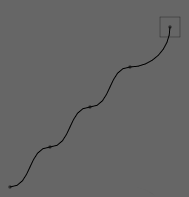
Let's build up a line with a few curved segments to show some of Field's operations that work on lines as a whole. For the purposes of this example, any old curve will do:
myLine = FLine()
myLine.moveTo(75,75)
for n in range(0, 4):
    myLine.polarCubicTo(1,-1, 1, Math.random(), 50+Math.random()*150,50+Math.random()*150)
Which gives, a random-ish set of curves:
First of all, we can copy this line, to get a completely independent line that contains all the same drawing instructions:
anotherLine = myLine.copy()
These two lines myLine and anotherLine are now independent. You can add things to each one of them and the other will not be altered in any way.
Given a line, we can translate it:
anotherLine += Vector2(30,0)
In this case 30 units to the right:
rotation() and .bounds()
Or we can rotate it:
anotherLine += rotation(Math.PI/2)
In this case 90 degrees (a.k.a. Pi/2) clockwise:
Rotation happens around some point. In the above example it's happening around the center of bounding rectangle that surrounds the FLine(). To rotate around some other point:
anotherLine += rotation(Math.PI/2, around=Vector2(0,0))
That's a rotation around the point 0,0 — the very top left of the canvas (unless, of course, you pan around the canvas):
Sometimes it's useful to pass in a function that returns the point you want to rotate around:
def aroundSomething(aLine):
    return aLine.bounds().topRight()

anotherLine += rotation(Math.PI/2, around=aroundSomething)
this can, of course, be more succinctly written:
anotherLine += rotation(Math.PI/2, around=lambda x : x.bounds().topRight())
Both these examples use the .bounds() method on FLine which returns a Rect that is the smallest rectangle that encloses the lines. Again, in this case, autocomplete / inspection on this Rect is the best way to go about seeing what methods you can call on it.
scale
scale() is just like rotation(), although here we use the = operator (scaling things is more like multiplication, translation is more like adding):
anotherLine *= Vector2(1, 0.5) # a non-uniform squish in the y-direction
anotherLine *= scale(0.5) # a uniform scale by 1/2 around the midpoint
anotherLine *# scale(0.5, aroundVector2(0,0)) # a uniform scale around the origin
anotherLine *# scale(0.5, aroundlambda x : x.bounds().bottomLeft()) # around the bottom left of the bounding box
It should be clear what these will do given the rotation examples above.
A general transform visitPositions
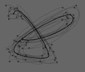
Sometimes you'd like to transform the content of the line in some other way. One way of doing this is visitPositions, which allows you to transform every point on the line with any given function. Thus:
def myFunction(x,y):
    return Vector2(x,y).noise(40)

for n in range(0, 10):
    anotherLine = myLine.copy()
    anotherLine.visitPositions(myFunction)
    anotherLine.color = Color4(0,0,0,0.2)
    _self.lines.add(anotherLine)
Or equivalently (with the use of Python's '''lambda'''):
for n in range(0, 10):
    anotherLine = myLine.copy()
    anotherLine.visitPositions(lambda x,y : Vector2(x,y).noise(40) )
    anotherLine.color = Color4(0,0,0,0.2)
    _self.lines.add(anotherLine)
visitPositions( lambda x,y : [...] ) applies the unction(x,y) that you pass in to every point (and every control point, if any) along the line and replaces its position with the Vector2 that this function returns.
The above code gets you something like:
A more specific transform visitNodes
visitPositions is very simple way of transforming a FLine, but it treats all data-points on the line the same — be they actual points on the line, or control points; be they straight lines or curved. And the result of filtering the Line is always a straight line if the original Line was straight and curved if it was curved.
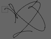
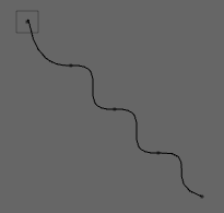
visitNodes gives us a little more control. Let's start with a line that has obvious sharp corners at its nodes:
myLine = FLine()
myLine.moveTo(80, 80)
for n in range(2, 6):
    myLine.polarCubicTo(1, -1.5, -0.5, 4.3, 40+n*40, 40+n*40)
Gives:
There's no simple function that you can pass into visitPositions that will smooth those kinks out, because to smooth this line you need to be able to shape the in and out cubic curve ''tangents'' at those points while keeping the actual positions along the line constant. There's no single transformation of all the points that does this.
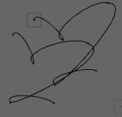
That's where visitNodes comes in. It takes a function that will be applied to each node in the FLine, and this function gets not just the position of the node, but the "before" and "after" points or control points (if they exist). It can modify any and all of these things by rewriting these variables. For example:
def nodeFunc(before, now, after, incomingCurve, outgoingCurve):
    tangent = ( (after or now)-(before or now) )*0.5
    if (before): before[:] = now-tangent
    if (after):  after[:] = now+tangent

myLine.visitNodes(nodeFunc)
Gives:
This sets the before and after tangents to be their average.
Note that the (after or now) construction ensures that this code works if after is None which will be the case at the end of the line. incomingCurve and outgoingCurve are set to 0 if before or after is coming from a control point or not.
A different angle on curve filtering visitPolar
Finally, while visitNodes is handy for modifying lines in cartesian space, sometimes you'd like to filter the ''direction'' that lines travel in. Since this can be a tedious piece of high-school trigonometry to craft by yourself, we have: visitPolar.
Let's start with a circle:
myLine = FLine()
myLine.circle(40, 150, 150)
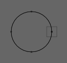
visitPolar takes a function to apply to each node in the line, just like visitNodes does. But its information is presented in a ''local polar coordinate'' system, specifically as an instance of a [source:/development/java/field/core/plugins/drawing/opengl/Polar.java PolarMove].
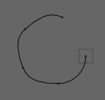
We can begin to unroll our circle a little:
def mover(move):
    move.alpha /= 1.3

myLine.visitPolar(mover)
which yields:
move.alpha is the angle turned by successive segments. Set it to 0 and you'll end up with a straight line (one that wiggles because the tangents are not straight, but progresses in a straight line nonetheless):
def mover(move):
    move.beta1 = 0
    move.beta2 = 0

myLine.visitPolar(mover)
beta1 and beta2 control the angle that the incoming and outgoing tangents make with the angle that the line is heading in. Set to `` we end up with something a lot more square:
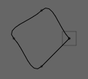
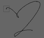
Correspondingly, rMain, r1 and r2 control the ''length'' of the new segment and its incoming and outgoing tangents. If you scale each of these things by two, in this case you end up with a circle that's twice as big. But do something a little different:
def mover(move):
    move.rMain *= 2
    move.r1 *= 2
    move.r2 *= -4

myLine.visitPolar(mover)
and you get something like this: