Images in Field

Field has quite a bit of support for drawing lines (and filled areas and points) — documentation is slowly growing at BasicDrawing. This is interesting for Field not just, or even mainly, because you can make art by drawing lines, but because having line drawing functionality available changes the nature of Field itself. With the addition of this functionality elements are free to articulate their own user interfaces, their own notations.

The Image handling features of Field are, at current, not nearly as disruptive as this. They are merely the result of a growing dissatisfaction we're having with piecing together workflows and prototype workflows out of bits of Photoshop, Illustrator, Final Cut / Motion and to a lesser extent SoundTrack. If we add the ability to load, display, manipulate and save images to Field then we can do our prototyping in the same place where we ultimately end up writing the "real" code. To this end, directly inspired by NodeBox, we have made a simple bridge between Field's drawing system and Core Image.

Tutorial

The FLine Image system is covered in this downloadable tutorial.

Hello Image

Loading an image is straightforward. Inside a new "Spline drawer" try the following:

from CoreGraphics import *
_self.lines.clear()
i = image("file:///Developer/Examples/OpenGL/Cocoa/GLSLShowpiece/Textures/Abstract.jpg")

(Remember, you can use command-" to get filename completion on such paths). Other kinds of URLs work as well, you could have written:

i = image("http://www.google.com/intl/en_ALL/images/cge_logo.gif")

Now to place it somewhere in the canvas:

i.show((100,200))

And there you go — an image in the canvas:

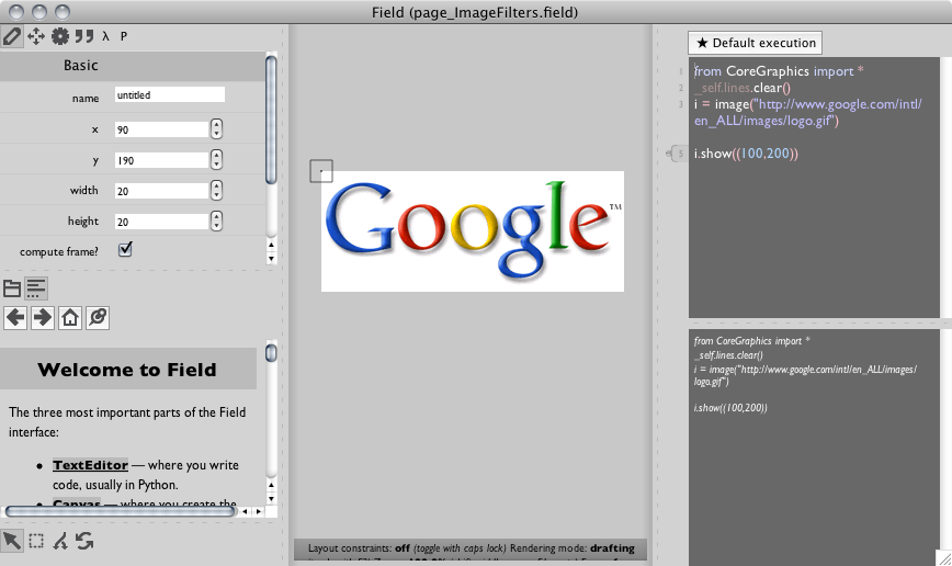
Field draws a rectangle around the image to help you locate images that have large areas of low alpha. To make this code steady state you'll want to add _self.lines.clear() at the top of your code: otherwise, as you keep execute this code, you'll end up accumulating more and more images on your canvas.

Hello Core Graphics

Apple's Core Graphics framework is the technology that does image processing (blurring, warping, leveling &c.) on OS X. Specifically, it uses the GPU to accelerate these operations. This means that under ideal conditions it's very fast. These "ideal conditions" include: a) never wanting to touch the results of computing image data with the CPU and b) being able to recast your image operations within the parallel programming paradigm supported by GPU's. If these two things are true then you are in for a Photoshop-beating treat.

Let's start simply: in Field, blur(5) in a convenient way of getting a blur filter (specifically a stock Apple CIGaussianBlur filter). Filters get applied to images using the << operator and this operation "returns" another image.

So, continuing with i as an image from the above example code:

(i<<blur(10)).show()

places a blurred version of the image on the screen:

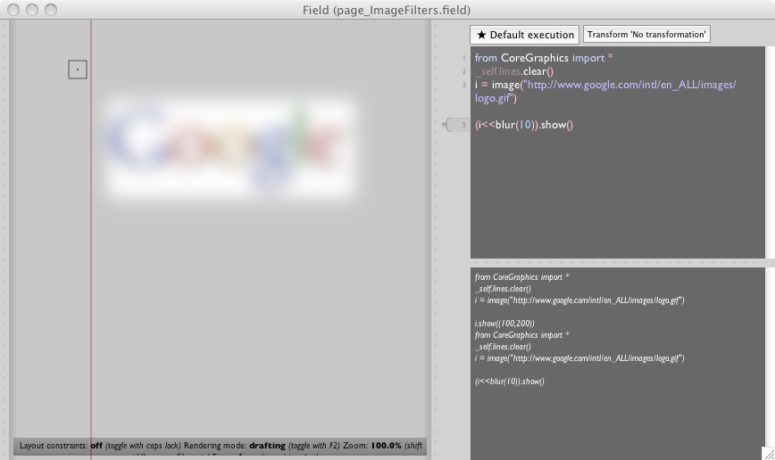
Two things to note: firstly images are immutable — they are never destroyed or modified — nothing has actually happened to the image i; secondly Field's bounding rectangles indicate both the extents and definition of the image, that is: both the region where one could expect to have any data and the (necessarily smaller or identical) region where one could expect to have completely determined data. The difference is apparent in this blur example. At the points that are closer to the edge than the radius of the blur we have feathering, until there's actually nothing left to blur.

Making a filter

OS X ships with a whole zoo of filters — specifically "Image Units" — and you can download more. The canonical reference for the "standard set" is here.

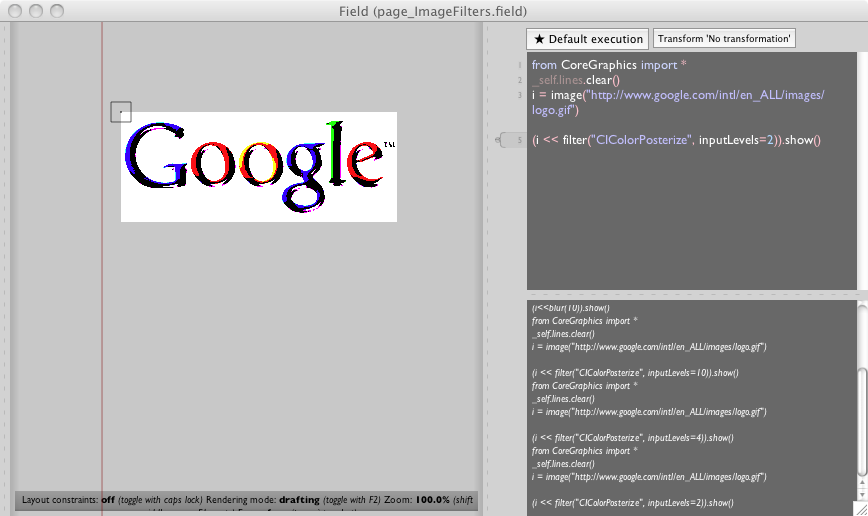
You can use this as a menu. Any of these these filters can be used within Field. Take for example, CIColorPosterize. Reading the documentation from above we see that it takes two "inputs": inputImage and inputLevels. In Field:

(i << filter("CIColorPosterize", inputLevels=2)).show()

this then gets you a very posterized image (posterized to 2 levels) on the canvas:

Three comments on the filter function. Firstly, it takes keyword arguments that correspond to the inputs talked about in the documentation. But unlike images, filters are mutable:

myPosterizer = filter("CIColorPosterize", inputLevels=10)
myPosterizer.inputLevels = 5

is perfectly valid. Secondly our << operator is just syntactic sugar for setting filter.inputImage # someImage and asking for filter.outputImage. Finally, you'll realize that blur(x) is now simply a short form for filter("GIGaussianBlur", inputRadiusx).

Making a filter, really

Choosing between Posterizing, Edge detecting or Cross-hatching an image is a little like rummaging through the Filters menu of Photoshop — fun for about half-an-hour when you are still learning how to use a mouse. While it's clearly superior to anything that Photoshop's scripting has to offer, writing it out in code doesn't have much more longevity. Core Image allows you to make your own filters using a programming language that Apple subsetted out of an industry standard (GLSL, short for GL Shader Language). The documentation for this language is here (and for GLSL, start here and proceed to the spec itself) but it's really best learned by example.

In Field:

myFilter = customFilter("""

kernel vec4 redScaler(sampler inputImage, float scale)
{
    return sample(inputImage, samplerCoord(inputImage))*vec4(scale,1,1,1);
}

""", [ "inputImage", "scale" ])

(i<<myFilter(scale=3)).show()

Some things to observe in the code above. This filter scales the red component of an image by its parameter 'scale'. Most of it is boilerplate: a declaration of the main function is prefixed by kernel. Nobody cares what it's called, but it takes two parameters: a sampler which gets you access to the input image and a float called "scale". The main body of the function samples from this image at the coordinate you'd expect (each input pixel maps to each output pixel) and takes this pixel-sample and multiples it by the 4-vector (scale, 1, 1, 1). And that's it.

The customFilter function returns a function that's just like filter but doesn't take the name of a "stock"-filter to look up. Currently it requires a list of the names of the parameters to the main kernel function, but I'm hoping to remove that parameter, or make it optional. customFilter ought to be able to parse the kernel declaration.

Now it's just between you and the documentation for the CIKernel language (ignore the parts about packaging up Image Units for use as plugins, Field makes it much easier than that to just write them in-place).

Making an accumulator

Apple's CoreImage framework defines one more useful thing that Field now supports — Accumulators. Core Image's images are typically secretly-lazily computed chains of filters (perhaps with some actual data at the very end of them). This framework works well for nested, branchy computation of filters — think the kind of non-linear, non-destructive editing in Aperture. It doesn't work so well for iterative techniques, one where you might apply a small number of filters a very large number of times to an image and never want to go back — think the kind of 'filter' that happens when you put down a brush stroke in Photoshop.

In Field, an accumulator you create an accumulator object with accumulator(x,y,w,h, isFloat) with the origin and dimensions, and whether or not the intermediate storage is floats (great precision) or bytes (speed). Accumulators look a lot like images:

#a 500x500 accumulator with floating point precision
acc = accumulator(0,0,500,500, 1)

i = image("file:///Developer/Examples/OpenGL/Cocoa/GLSLShowpiece/Textures/Abstract.jpg")

#copy the image 'i' into the accumulator directly
acc <<= i

#blur it over and over again (takes around 0.5 seconds on my GeForce 8800)
for n in range(0, 100):
    acc <<= blur(10)

#put it on the screen
acc.show( (40,40) )

One difference you'll find is that since Accumulators are mutable, you can put them on the canvas (via show) once and they'll update without you doing anything to reflect their current contents.

Under the hood

But in either case, just what is i.show() doing? How are these images being shown? The answer is that Field's line drawing system has been extended to understand how to show Core Graphics images. Just as the following code displays some text:

_self.lines.clear()

line = FLine().moveTo(40,40)
line.containsText = 1
line.text_v = "hello world"

_self.lines.add(line)

This code displays an image:

_self.lines.clear()

line = FLine().moveTo(40,40)
line.containsImages = 1
line.image_v = image("/Developer/Examples/OpenGL/Cocoa/GLSLShowpiece/Textures/Abstract.jpg")

_self.lines.add(line)

This means, by the way, that you are free to grab that point with the mouse drag it around and allow it to be affected by a subsequent _self.tweaks() statement — see BasicDrawing for more information.

Rasterization

While the image drawing facilities are cunningly embedded inside the line drawing facilities, that doesn't really count as integrating them. This is hard-ish to do: Field has its FLines and OS X and Core Graphics and Quartz have their own NSBezierPaths and CGPaths and things, both ideas of lines overlap but are tightly integrated into the libraries that "own" them. Bridging them is tedious and error prone, and Apple is being no help at all right now.

But we can avoid this whole hard-ish thing, at the expense of recalculation-speed by exploiting Field's PDF export abilities. Nobody will want to do real-time animation this way, but for exploring hybrid vector / pixel image making, this is probably fast enough.

The Core Graphics extensions to Field defines a new function rasterizeLines() that takes a list of FLines (or pulls them out of _self.lines) and optionally a bounding box (defaults to the bounding box of its inputs), optionally a background color (defaults to transparent), and optionally a scale (defaults to 1.0) and returns an image with those lines rasterized by the Quartz/PDF drawing path. The "default" location of the image (where it ends up if you just write show() is set to be the spot that overlaps with the lines that were there to generate it. This is slow (as in 100s of milliseconds slow, not go-away-and-have-a-coffee-slow) but very high quality.

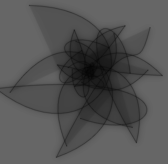
The following code then makes a arbitrary and pretty (and very 'vector') mouse editable Bezier-doily and effectively gives it a soft drop shadow:

_self.lines.clear()


for n in range(0, 10):
    d = FLine()
    d.moveTo(n*4, n*3)
    d.cubicTo(n*3, n*2, n*2, n*3, n*5, n*4)
    d.cubicTo(n*4, n*2, n*2, n*4, n*4, n*5)
    d*=Vector2(24.0,23.0)
    d+=rotation(1*n)
    d+=Vector2(100,500)
    d.color=Vector4(0,0,0,0.75)
    d.thickness=1
    d.fillColor=Vector4(0,0,0,0.05)   
    d.filled=1
    _self.lines.add(d)


_self.tweaks()

i = rasterizeLines(_self.lines)

(i<<blur(3)).show(decor=0)
(i<<blur(13)).show(decor=0)

Yields:

Note: the scale parameter to rasterizeLines() (see the auto-complete) is very useful if you are ultimately exporting pdfs that contain images for the purposes of printing or you have zoomed your canvas in close, since the default scale=1.0 is effectively screen resolution at the default zoom level (e.g. 72dpi).

Raw access to those Pixels

Core Graphics doesn't want you to be able to set or get individual pixels. This is very much in line with the way that graphics APIs and hardware has been heading in the last decade. You configure a high level, and elaborate "form" for the rendering — using a very subtle and complex API — and then just tell a piece of hardware to "go execute it and put it on the screen" in as simple (and as fast) a way as possible. Playing at the pixel level doesn't fit well within this scheme.

But sometimes you have to deal with raw pixels. Two common situations where this is the case. Firstly, when you actually have some raw pixels you want to put on the screen: perhaps the result of some computation, or something that needs visualizing (a sound file perhaps?). Secondly when you want to obtain "an answer" back out of a computed image, quite possibly some statistics over an image or an image area.

We'll take these cases in order.

Originating Pixel data

We've seen in the above example code that the image class takes a string as its constructor parameter. There's another form: one that takes a FloatBuffer (as in a java.nio.FloatBuffer) and a width and a height. Right now this float buffer is expected to be an array of floats, row by row, in "red, green, blue, alpha" format. Because of the intrinsic immutability of images, if you want to update the image after updating this float buffer, you'll need to go get a new image instance.

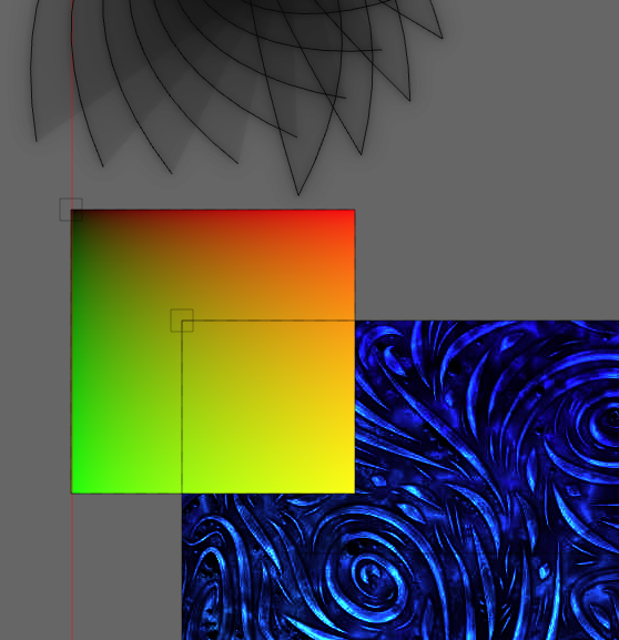
Here, a slow way of making a gradient from red at the top left to yellow at the bottom right:

imageData = makeFloatImageData(256, 256)
for y in range(0, 256):
    for x in range(0, 256):
        imageData.put(x/256.0)
        imageData.put(y/256.0)
        imageData.put(0.0)
        imageData.put(1.0)

ii = image(imageData, 256, 256)
ii.show()

Yields:

If you plan to frequently change this gradient (or make it much larger) then, in this specific case you'd be much better served either reading the documentation for CILinearGradient or, in general, writing this code in the CIKernel language. But if it's just a static image (used elsewhere in the computation) then once it's computed, it's as fast to use as any other image.

Getting Pixel data back

How about getting the pixel data back? Firstly, stop. Do you really want to get the pixels back? Are you sure that you don't just want to a) save them to disk (consider image.savePNG(filename)) b) get some statistics about them (consider filter("CIAreaHistogram" ... ) or CIRowAverage or the like)?

CIAreaHistogram can be very useful. For example, using the new MinimalImageHistogram embeddable UI we can recreate Photoshop's levels control:

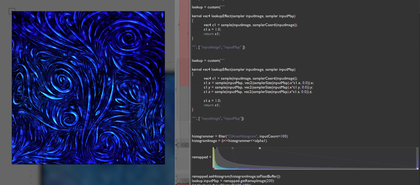
But I digress, perhaps you really want to force the data to swim all the way upstream, in the wrong direction, from the graphics card to the CPU. In that case:

i.toFloatBuffer()

This returns a FloatBuffer (again, as in java.nio.FloatBuffer) that contains the "red,green,blue,alpha" row by row data for the image. Write to this FloatBuffer and nobody will notice — you'll have to make a new image (see the section above). To access this this buffer intelligently you'll need to know its width: i.getExtents().w.

For example, this gets you to the pixel data itself:

from CoreGraphics import *
from java.awt import Color

ii = image("/Users/marc/Desktop/testImage.jpg")

_self.lines.clear()

ii = ii <<blur(10)

ii.show()

w = int(ii.extents.w)
h = int(ii.extents.h)

fb = ii.toFloatBuffer()

def getPixel(x, y, floatBuffer, w, h):
    r = fb.get(4*w*y+4*x+0)
    g = fb.get(4*w*y+4*x+1)
    b = fb.get(4*w*y+4*x+2)
    a = fb.get(4*w*y+4*x+3)
    # float constructor for Color, values above are premultiplied
    if (a>0):
        return Color(r/a,g/a,b/a,a) 
    else:
        return Color(0,0,0,0)

getPixel(100,60, fb, w, h).getAlpha()

Issues & Goals

These Core Graphics "extensions" are pretty fresh, and they contain a number of clear limitations. The largest is that it leaks memory. It leaks less than it used to, and it's small enough that you can still get serious work done with it, but occasionally it seems to have a few issues. Tracked as ticket, #39.

Leaking memory is invisible (if you have enough memory), but the most visible limitation is that the core graphics images attached to points inside the line drawing system don't persist with the Sheet, they need to be recomputed when the sheet opens (you can always stick your code in python_autoExec_v). I'm a little torn — not, about how to implement this, but whether we should — including the such image assets inside the sheet folder directly seems like it will make the sheets rather large very quickly (should they even get versioned?).

A sustained example

I'd like to append to this tutorial some longer source code (the origin of which is explained in our main-site blog posting). This is the source code to a "healing brush" like algorithm. There's no "brush", rather a separate mask image (as if the brush had brushed black on a white background), and a constant offset to where the "source area" comes from. The goal of this approach is to "in-paint" an image that's missing a whole (missing, that is, the area "brushed out" in the mask) by copying the texture from the "source area" but manipulating the colors and the color gradient to make the edit appear seamless. It seems to produce results largely equivalent to the tool in Photoshop.

I'm including it here not just because both academics and companies get to write about code without sharing code, but because it's a fine example of code thats particularly easy to write in Field, because, as you are writing it, it's easy to build it up incrementally. Testing, analysis and writing code become one.

first the standard introduction:

from CoreGraphics import *
_self.lines.clear()

now, some images. The image we'll be in-painting:

i = image("file:///Users/hb/Documents/possionInput3.tif")
(i).show((100,100))

and the mask which will mark the area to be in-painted (this doesn't have to be black / white, it can have grey in it)

m = image("file:///Users/hb/Documents/mask3.tif")

The basic trick is to run the in-painting algorithm on shrunken version of the image first and to get approximate solutions to less shrunken images which then get refined and so-on, all the way back to the original resolution:

#function to construct a pyramid of successively smaller images
def constructImagePyramid(input):
    images = []
    w = input.getExtents().w
    h = input.getExtents().h       
    while (w>1 and h>1):
        images.append(input)
        input = (input*0.5)
        w = input.getExtents().w
        h = input.getExtents().h   
    return images

To do the "smoothing", we'll need some custom Core Image filters:

#simple smoother
lapsmooth = customFilter("""

kernel vec4 smoother(sampler inputImage)
{
    vec4 s1 = sample(inputImage, samplerCoord(inputImage)+vec2(-1,0) );
    vec4 s2 = sample(inputImage, samplerCoord(inputImage)+vec2(1,0) );
    vec4 s3 = sample(inputImage, samplerCoord(inputImage)+vec2(0,1) );
    vec4 s4 = sample(inputImage, samplerCoord(inputImage)+vec2(0,-1) );

    vec4 o =  (s1+s2+s3+s4)/4.0;
    o.w = 1.0;
    return o;
}

""", [ "inputImage" ])

#a more complex smoother that takes into account the gradient information of some other image
gradientSmoother = customFilter("""

vec4 gradientAt(sampler from, vec2 direction)
{
    vec4 s1 = sample(from, samplerCoord(from));
    vec4 s2 = sample(from, samplerCoord(from)+direction);
    return s2-s1;
}

kernel vec4 smoother(sampler inputImage, sampler gradientImage)
{
    vec4 s1 = sample(inputImage, samplerCoord(inputImage)+vec2(-1,0) );
    vec4 s2 = sample(inputImage, samplerCoord(inputImage)+vec2(1,0) );
    vec4 s3 = sample(inputImage, samplerCoord(inputImage)+vec2(0,1) );
    vec4 s4 = sample(inputImage, samplerCoord(inputImage)+vec2(0,-1) );

    vec4 d1 = gradientAt(gradientImage, vec2(-1,0));
    vec4 d2 = gradientAt(gradientImage, vec2(1,0));
    vec4 d3 = gradientAt(gradientImage, vec2(0,1));
    vec4 d4 = gradientAt(gradientImage, vec2(0,-1));

    vec4 o =  (s1+s2+s3+s4)/4.0;

    vec4 d =  (d1+d2+d3+d4)/4.0;
    o+=d;

    o.w = 1.0;
    return o;
}

""", [ "inputImage", "gradientImage" ])

And a utility filter (I'm sure I could get this from a stock CIFilter, but it's faster to write this than it is to look it up:

#just shoves an image over, by default we take our clone area to be a constant offset from points to remove

offseter= customFilter("""

kernel vec4 offseter(sampler inputImage, vec2 offset)
{
    vec4 s1 = sample(inputImage, samplerCoord(inputImage)+offset);
    s1.w=1.0;
    return s1;
}

""", [ "inputImage", "offset" ])

Finally, we run the smoothing over the entire image, but only apply the results to the part given by the mask.

# for the Laplacian solver to iterate only inside the areas to remove
maskedReplace = customFilter("""

kernel vec4 smoother(sampler inputImage, sampler original, sampler mask)
{
    vec4 i = sample(inputImage, samplerCoord(inputImage));
    vec4 o = sample(original, samplerCoord(original));
    vec4 m = sample(mask, samplerCoord(mask));

    vec4 a = mix(i, o, m);
    return a;
}

""", [ "inputImage", "original", "mask" ])

And, at last, definitions over, the code itself.

# the brushstroke offset (it's important that this is still on-screen)
offset = Vector2(-40,40)

# get a pyramid of the main image
pyr1 = constructImagePyramid(i)

# get a pyramid of replacement material
pyr2 = constructImagePyramid(i<<offseter(offset=offset))

# smooth our mask a little
for n in range(0, 8):
     m = m<<lapsmooth()

#a pyramid of the mask
pyrMask1 = constructImagePyramid(m)

#the algorithm itself (we should recode this using Accumulators, see above)
def multigridGradientLaplace(imagePyramid, gradientImage, maskPyramid):
    nextImage = []
    for n in range(len(imagePyramid)-1, -1, -1):
        for q in range(0, 5):
            smoothed = imagePyramid[n]<<gradientSmoother(gradientImage=gradientImage[n])
            imagePyramid[n] = smoothed<<maskedReplace(original=imagePyramid[n], mask=maskPyramid[n])
        if (n>0):
            expanded = imagePyramid[n]*2
            imagePyramid[n-1] = expanded<<maskedReplace(original=imagePyramid[n-1], mask=maskPyramid[n-1])

#actually call the algorithm
multigridGradientLaplace(pyr1, pyr2, pyrMask1)

#and put the result onscreen
_self.lines.clear()
pyr1[0].show( (700, 0) )

The result, given a suitable mask, which loosely marks the area to remove:

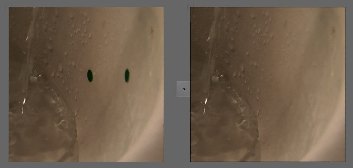
There — hardware accelerated marker and line removal, built iteratively and visually, in a page of code.