
Simulations deep and wide
This page covers four useful additions to Field that fall under the umbrella of “simulation” — simulation of Physics in 2 dimensional worlds; the simulation of simple flocking behaviors (of birds and fish, or, at the very least, robotic birds and fish); a canonical piece of “experimental math” that builds natural shapes like tress and snowflakes and, finally, when all else fails, and physics and mathematical descriptions of the complexity of nature escape your — random numbers
2D physics
The first, and perhaps the most generally useful, is a general purpose 2D physics engine. This is actually an implementation of a popular physics system called Box2D that has been used in a wide variety of computer games over the last 10 years or so. If you’ve “Cut the Rope” or Angered a Bird in any way on a phone you have interacted with this particular very engine.
As all physics engines do we combine three things which, taken together, cover much of what we mean by “physics” for a 2d world: motions on bodies controlled by forces and torques, collisions that end up applying forces and torques to those bodies in motion and joints that couple and constrain the motion of bodies. Here, in Field, “body” is an FLine.
Let’s start, as usual, with some example code:
A jittery square
_.lines.clear()
var f1 = new FLine().rect(10,10,100,100)
f1.color=vec(0,0,0,1)
f1.filled=true
_.lines.f1 = f1
This should come as no surprise:
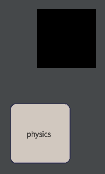
Up until now if we wanted this line to move we might have some kind of a loop:
while(true)
{

	// do something great to f1
	_.lines.f1 = f1 + vec(0,0).noise(10)

	_.redraw()
	_.wait()
}
This would cause f1 to jitter around randomly.
Rather than doing that, let’s add some physically simulated motion to that FLine called f1:
A spinning square
// 1. make a new Physics System
var PhysicsSystem = Java.type("trace.physics.PhysicsSystem")
var p = new PhysicsSystem()

var f1 = new FLine().rect(10,10,100,100)
f1.color=vec(0,0,0,1)
f1.filled=true
_.lines.f1 = f1

// 2. add physics to the line f1
p.addPhysics(f1)

// 3. apply a torque to our FLine
f1.physics.applyTorque(1000)

while(_.wait())
{
	// update the physics world and any FLine attached to it
	p.update()
	_.redraw()
}
We’ve added four things to our standard drawing of a rectangle. First, we’ve made a PhysicsSystem which is a ‘world’ for (simulated) physical bodies to interact in. FLines can participate in at most one PhysicsSystem. Secondly, we associate an FLine with this particular PhysicsSystem called p with the line p.addPhysics(f1). Thirdly we’ve applied a torque to the FLine (torque being the precise word to talk about a purely rotational force). We do this by calling applyTorque on f1.physics. f1 got a .physics from our call to addPhysics. Finally we have an animation loop that called p.update() — this gives the PhysicsSystem a chance to compute the next step of what the world looks like and modifies the line f1 to follow the trajectory given by its forces and torques.
What do we get from all of our effort? This:
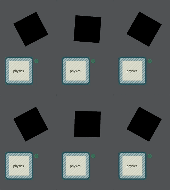
We’ve applied a ‘push’ to our rectangle and sent it spinning, but the actual spinning comes from the physics simulation. As typical, we can take this much further.
A spinning, falling, colliding square
// three rectangles ---
var PhysicsSystem = Java.type("trace.physics.PhysicsSystem")
var f2 = new FLine().rect(200,200,100,100)
var floor = new FLine().rect(0,500,500,10)

f1.color=vec(0,0,0,1)
f1.filled=true
_.lines.f1 = f1

f2.color=vec(0.2,0,0,1)
f2.filled=true
_.lines.f2 = f2

floor.color=vec(0.2,0.2,0.2,1)
floor.filled=true
_.lines.floor = floor

// add physics to all three of them --
var p = new PhysicsSystem()
p.addPhysics(f1)
p.addPhysics(f2)
p.addPhysics(floor)

// make sure that the 'floor' isn't allowed to move
floor.physics.setFixed()

// send the first one spinning
f1.physics.applyTorque(1000)

// set the other one gliding over to the left
f2.physics.applyForce(vec(-20,0))

// and, while we're here, add some gravity to everything (that points 'down')
p.setGravity(vec(0,1))

// and, again, update the physics system while redrawing frames
while(_.wait())
{
	p.update()
	_.redraw()
}
This gives us a more complex toy-box:
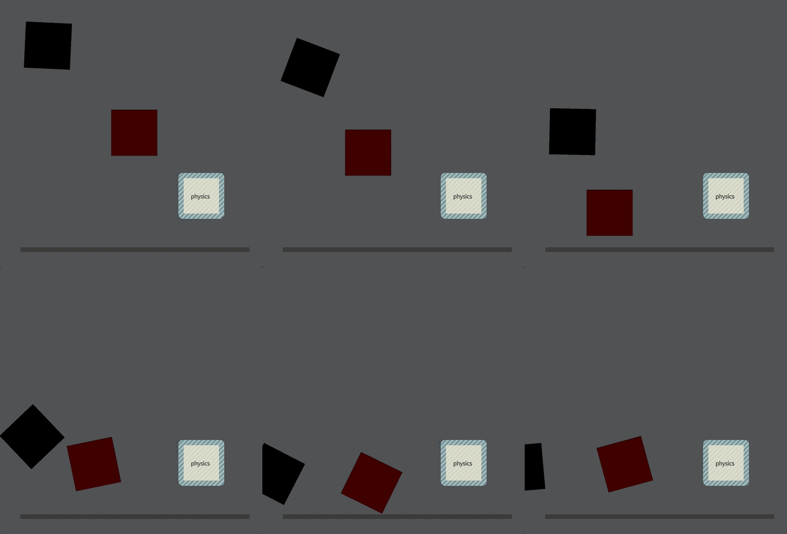
We see here behavior that would be incredibly tedious to plot out by hand: the fall of the red box inscribes a parabola (which is what falling / moving objects do in the ‘real world’), until it bounces then collides partially with the black box, and they both spin and slide convincingly. The motion is detailed and believable. This is parametric motion — if we want to move the box over a little, we just move the box over a little and the computer computes the new motion.
There is a range of things that you can call on these physics objects that attach themselves to FLines once you have called addPhysics:
The physics engine
applyTorque(x)— adds a rotational forceapplyForce(vec(x,y))— adds a translational forcesetLinearVelocity(vec(x,y))— sets the velocity (that’s direction and speed) of an object.setRotationalVelocity(x)— sets how fast the object is spinning/setDensity(x)— sets the density of objects, how much they ‘weight’ per how big they are.setFixed()— makes the object not move under any circumstances (although it still can participate in collisions).setRestitution(0.3)— determines how ‘bouncy’ or elastic an object is (note, this is ultimately a combination of both things that collide). Default to 1 (like a rubber ball)setFriction(0.8)— determines how quickly touching objects grind to a halt if they keep touching. Defaults to 0 (like wet ice on wet ice…).
Finally, two things that you can do with the physics system itself:
p.setGravity(vec(x,y))— sets a gravity direction (where things fall). Remember ‘y’ points down in Field, therefore you’ll want a gravity likevec(0,10).p.distanceJoint(someFLine, someOtherFLine)— makes a joint between the centers of twoFLinethat tries to keep the distance between them fixed, like a spring.p.distanceJoint(someFLine, someOtherFLine, dampingRatio, frequency)— likedistanceJointbut with more control over how much the physics system will try to maintain the joint. For examplep.distanceJoint(f1, f2, 0.01, 10)will produce a much stiffer (potentially to the point of instability) joint.p.weldJoint(someFLine, someOtherFLine, dampingRatio, frequency)— like a distance joint, but also maintaining (or trying to maintain) rotational constraints as well.
Contact Events
Once (but not before) you’ve called addPhysics on an FLine you can also ask for contact events. This lets you arrange for pieces of code to be called when objects hit other objects. A collision has a start and (possibly) an end. Here’s how to change the color of that line f2 above when it’s in contact with something else:
The beginnings of gameplay
f2.onContactStart.someCallback = (other, points) =>
{
	f2.color=vec(1,0,0,1)
}

// 'someCallback' is just any name, this is working like
// _.lines.someCallback = new FLine() would work
f2.onContactEnd.someCallback = (other) =>
{
	f2.color=vec(1,1,0,1)
}
That will set f2 to be bright red when it’s in contact with anything else, and then yellow when that contact stops:

If want to get extra fancy, you can use the parameter other that’s passed into that function to change this behavior based on the other FLine that this FLine is hitting. Note, also, that there’s a parameter points that’s passed into the onContactStart function. This contains a list of points where the contact is occuring.
Limitations
Things to watch out for
And, two cautionary notes:
- This Box2D won’t draw / collide curves properly — it will just use a straight line. You can use geometry more complex than mere rectangles, but if you want to collide curvy things together then you might want to subdivide them first (and thus get a lot of small straight lines).
- Things get their masses from their density multiplied by their size — A torque of ‘100’ when applied to a large rectangle will spin it much less than a small one, because a large rectangle is much heavier. The default density is 0.0001 units (specifically Kg per cubic pixel).
A full 2D physics interface reads longer than this — you can vary the coefficients of friction and the elasticity of objects for example and there are many, many more kinds of joints — but it isn’t more complex. We have the fundamentals here, and we always extend this out further if final projects demand. Finally, we should note that typical computer have enough computational power for around 100 potentially colliding objects. For example, if we add this to the above example:
A sandbox of boxes
for(var i=0;i<100;i++)
{
	var f = new FLine().rect(Math.random()*500, Math.random()*100, 10, 10)
	p.addPhysics(f)
	_.lines.add(f)
}
We get:
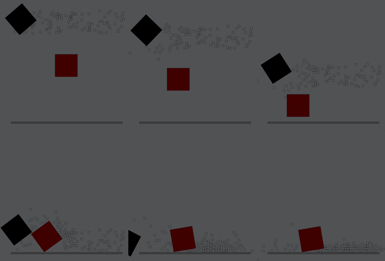
(You can see some jumping about at the beginning because some of these random rectangles end up inside the larger rectangles so they are quickly pushed out).
Prompts:
- Remember that you can add
FLines to the physics system without drawing them and, rather, use whereFLines end up after physics is updated to draw something else - Try driving physics objects from motion capture traces.
- How would you implement ‘squash and stretch` ?
Boids
The second “simulation” addition to Field this week is a Boids model. Boids is a ‘famous’ model that reproduces a range of flocking-like behavior that seems to mimic some of the properties of aggregations of animals (from birds to slime molds). There’s much information to be had out of Craig Reynolds’ website who was probably the first to formally realize the generative potential of the approach. Ultimately, we’ll let the example code speak for itself:
A Flock of Boids
// make a new Boids simulation
var Boids = Java.type("trace.physics.Boids")
var boids = new Boids()

// add 120 boids that all start at a random position, head in a random direction and move with speed '1'
for(var i=0;i<120;i++)
	boids.addBoid(vec(0,0).noise(100), vec(0,0).noise(1), 1)

// configure the simulation to say that '4' units is 'too close'
boids.tooClose=4

// but 10 units is too far
boids.tooFar=10


// here's our animation loop
while(_.wait())
{
	// update the boids simulation with speed 1
	boids.update(1)

	// and now we just draw the boids
	var f = new FLine()

	// for each boid
	for(var bb of boids.all)
	{
		// make a rectangle, rotate it to match the boid and move it to the correct spot
		f.append(new FLine().rect(-2,-2, 4,4) * bb.rotation() + bb.at)
	}

	_.lines.f = f
	_.redraw()
}
This yields something that’s eerily like a flock of birds:
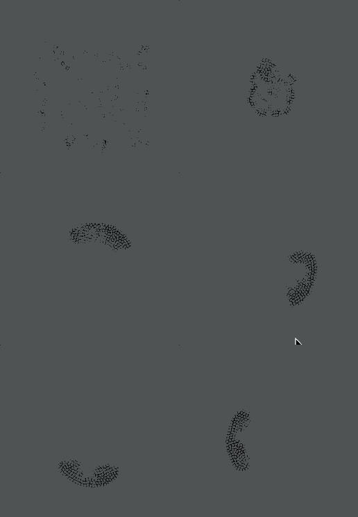
Highlights from the code above:
bb.atis avec(x,y)that tells you where the boid is. You can set this to something else if you like, for examplebb.at.x = 30and the boid will be teleported therebb.rotation()— returns something that will rotate anFLineto have the same heading as a boidbb.bb.tooCloseandbb.tooFarcontrol the simulation parametersboids.addBoid(startingPosition, startingHeading, speed)adds a boid to simulationboids.allis a list of all of the boids in a simulationboids.headBoid(index, position, heading)— nominates, for this single frame only, boid numberindexhas really important, teleporting it topositionwithheading.
Prompts:
- (Radically) different ways of drawing the “colony” — (clue: one of the strategies in the BIPED movie for controlling the vertical lines was effectively Boids)
- Different speeds of boids
- Strategies for resetting or seeding the positions of the Boids — seed Boids from a piece of geometry then map the geometry back onto the Boids?
L-Systems
L-Systems are a “notational / computational” system that we saw briefly when we looked at notational strategies. Really, they straddle notational concerns (they build micro-languages for describing drawing processes), and simulation concerns (the arise out of trying to build geometries that seem organic and grow organically). Like ‘Boids’, you can do worse than simply Google them.
A general ‘production system’ (which is the fancy name for the family of languages that L-Systems are a part of) combines three things which act on “sentences” made up of letters. The first is the ‘axiom’ — which is simply the starting sentence. The second is a set of ‘production rules’ that, when they match parts of a sentence rewrite that part to be different. Finally, there are a set of rules that interpret what the letters mean or do — usually, in our case, to issue some instructions into an FLine.
Let’s go:
// make a new production system
var Production = Java.type("trace.physics.Production")
var p = new Production()

// add two rules
// 0 -> 10
// and
// 1 -> 0[1][0]

p.addRule("0", "10")
p.addRule("1", "0[1][0]")
Our rules say, wherever you see ‘0’ replace it with ‘10’ and wherever you see ‘1’ replace it with ‘0[1][0]’. We don’t need to use ‘0’, ‘1’, ‘[’, or ‘]’, we are free to use any characters we want. We can also have rules that match more than one character, like ‘01’ -> ‘0AB1’.
Now we can run our production system a little and see what it grows:
var q = "0"
for(var i=0;i<3;i++)
{
	q = p.apply(q)
	print("stage "+i+" is "+q)
}
This will print something like:

As you can see the ‘sentence’ grows quickly from ‘0’ (often you’ll find that you can run this loop with more than, say, 7 iterations).
So far we’ve played a ‘syntactical’ substitution game; let’s add some semantics - what the letters mean:
var f = new FLine()
f.moveTo(0,0)
_.lines.f = f

p.addAction("0", () => {
	f.lineForward(10)
})

p.addAction("1", () => {
	f.right(4)
	f.lineForward(20)
	f.left(4)
})

p.addAction("[", () => {
	f.left(1)
	f.push()
})

p.addAction("]", () => {
	f.pop()
})
These ‘rules’ say, whenever you see ‘0’ do f.lineForward(10) (which adds a line in the ‘forward’ direction). Calls like f.right(4) rotate our ‘heading’ by 4 degrees to the right.[ and ] save and reload the position and direction of the line respectively.
One final call applies these action rules to the sentence that we built:
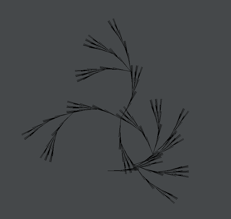
p.act(q)Yielding this shape here:
As usual there are a number of routes in here.
- Change the action for ‘[’ to include a
_.wait() _.redraw()or a_.stage.frame()and watch the tree draw out. - Explore different micro-languages.
- Decorate this tree with more lines than this.
- Animate those angles over time.
Random
The last useful ‘simulation’ we’ll add to Field is a class of random number generators. True randomness is something that computers, the story goes, find particularly hard. In truth, for all of our purposes, computers have no trouble producing completely unpredictable number sequences. The trouble, rather, is that we don’t want completely unpredictable number sequences. Rather we go to “random sequences” when we want things to look less like a computer made them.
Partially in response to this desire to produce “organic” sequences of numbers — that is, variations that wobble in the ways that natural phenomenon wobble — Ken Perlin came up with a new approach to randomness in the early 80s. Fast to compute, easy to control, the approach has been used widely to ‘rough up’ almost everything that might otherwise seem sterile: textures (to make things look less computer generated), motion (to make things look less robotic), rhythms (to make things sound like a ‘real’ drummer) etc. It’s in Toy Story (the wood textures), it’s in Tron (the geometry of the rock / ice formations) and there’s nary a CGI tree that waves in the wind that isn’t waving to Perlin’s function and so on. Once you start to see it, it’s everywhere. So much so, in fact, that Perlin won a technical Oscar for what amounts to a single mathematical function.
Let’s motivate it this way. First of all, let’s begin with the noise function that many of you have been using to date Math.random()
var f = new FLine()

for (var i=0;i<5000;i++)
{
	var v = Math.random()

	// scale it so we can see it:
	f.lineTo(i, v*100)
}

_.lines.f = f
This plots something like this:

Math.random() returns a random number between 0 and 1. Other than the many many more numbers involved, this is a lot like tossing a coin: each number is completely independent from the one before. There are lots of ‘grade school math’ tricks to shape this randomness. For example:
var f = new FLine()

for (var i=0;i<5000;i++)
{
	var v = Math.random()

	v = v*v*v*v*v

	// scale it so we can see it:
	f.lineTo(i, v*100)
}

_.lines.f = f
This makes the randomness ‘spikey’ for example. (You might work through this in your head: raising numbers between 0 and 1 to large powers makes most of them all much closer to 0, leaving only a handful that happened to be very close to 1 spread out over the rest of the range).
But functions of a single random value like this are at best a crude way of manipulating how this change varies over time. And it’s not completely clear how to proceed. If we want something that’s “smoother”, we could start to play games like this:
var f = new FLine()

var lastValue = 0

for (var i=0;i<5000;i++)
{
	var v = Math.random()

	lastValue = lastValue * 0.9 + 0.1 * v

	// scale it so we can see it:
	f.lineTo(i, lastValue*100)
}

_.lines.f = f
Yielding:

This builds a sequence where the ‘next’ number is 90% the same as the previous number, 10% random. We can continue, for even less wiggle, even more ‘smoothness’ with a 99% and 1%:
var f = new FLine()

var lastValue = 0

for (var i=0;i<5000;i++)
{
	var v = Math.random()

	lastValue = lastValue * 0.99 + 0.01 * v

	// scale it so we can see it:
	f.lineTo(i, lastValue*100)
}

_.lines.f = f
Yielding:

As you can see this certainly is smoother, but it doesn’t really wobble at all. In fact the only real long term change is because we’ve picked the wrong first value for this function (var lastValue = 0) if we change that to var lastValue = 0.5 we’ll see that there’s hardly any variation to this line. We’ve tried to change the ‘frequency’ and the amplitude has changed as well.
We want something that still wiggles as much as ever, as much as the original pure Math.random() function, but wiggles slower — not to fast, not too slowly. This is Perlin Noise:
var f = new FLine()

var random = new Random()

for (var i=0;i<5000;i++)
{
	var v = random.nextDouble(0.1)

	// scale it so we can see it:
	f.lineTo(i, v*100)
}
 —
_.lines.f = f
This gives this, very different function:

First of all it’s between -1 and 1, but unlike our attempts at smoothing Math.random() it really does fill this range. Secondly is moves much slower. That’s controlled by the parameter to nextDouble(0.1). Setting that to nextDouble(0.01):

That parameter roughly controls the frequency of the noise — small numbers yield slow functions, numbers beyond and including 1 give us Math.random() again. We can do things like this:
//...
	var v = random.nextDouble(i/10000)
//...
And watch our wobble ‘ramp up`:

Random cascades
Perlin noise is a very useful building block to build organic feeling things. In a loose sense, a Perlin noise function yields a random sequence that has frequencies within a single ‘octave’. The first move towards building more complex random sequences is usually to combine Perlin noise functions at different octaves and amplitudes together. We end up with more control because we can vary the amplitudes of each octave separately. This is such a useful approach that it’s also built into Field:
var f = new FLine()

var random = new RandomCascade()

for (var i=0;i<5000;i++)
{
	var v = random.nextDouble(0.05)

	// scale it so we can see it:
	f.lineTo(i, v*100)
}

_.lines.f = f
Yields:

This has just a little more small, high-frequency wiggle, on top of lots of low-frequency wobble. Functions like these turn up everywhere in nature. For large chunks of ‘time’, musical instruments are like this, variations in the tides are like this, the stock market is like this (except when they aren’t). RandomCascade is adding together 4 Randoms at 4 different ‘octaves’ in proportions 1, 1/2, 1/4, and 1/8. We can configure this:
random.a[3]=0.2
random.h[3]=16
random.a[2]=1
random.h[2]=0.1
This sets the amplitude of the 4th noise function a[3] to 0.2 and the frequency h[3] to 16x while setting the third noise function to 1 and it’s frequency to a very slow 0.1x. This gives:
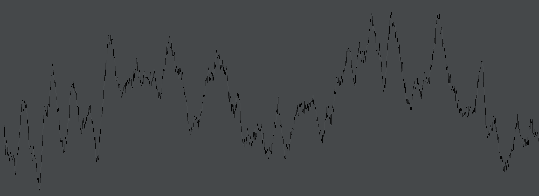
Which recalls that stock market (on a normal day) or a mountainside.
Events
Once we have a smoothly varying random function we can use that to drive other “random” processes. Here’s an important strategy:
var f = new FLine()
var events = new FLine()
events.color = vec(1,1,1,1)

var random = new RandomCascade("seed", 2)

var lastValue = 0

for (var i=0;i<5000;i++)
{
	var v = random.nextDouble(0.1)

	if (v<=0 && lastValue>0)
		events.moveTo(i, -100).lineTo(i, 100)

	f.lineTo(i, v*100)

	lastValue = v
}

_.lines.f = f
_.lines.events = events
This turns out random ‘events’ (white lines) that have random, but controllable frequency (they are generally never too close and never too far apart):

Reproducibility
One final note: Randomness is sometimes exactly what we need to catch sight of something interesting. Don’t know how to make something move? wiggle it with a random function. Don’t know what color to make something? Add Perlin Noise. One trick, though, is to be able to reproduce your discoveries. Random and RandomCascade come with alternative constructors that let you seed your random functions. Given the same seeds, you’ll get the same random sequences.
Here’s the syntax:
var random = new Random("seed", 2)If you change “seed” to something else, or that 2 to any other number you’ll get a completely different sequence of random numbers out, another (Perlin) set of random dice rolls. But if you don’t change it, your code will always reproduce what it did last time.